TECHNICAL PAPER

 

Pile design practice in southern Africa Part I: Resistance statistics

 

 

M Dithinde; J V Retief

Contact details

 

 

---

ABSTRACT

The paper presents resistance statistics required for reliability assessment and calibration of limit state design procedures for pile design reflecting southern African practice. The first step of such a development is to determine the levels of reliability implicitly provided for in present design procedures based on working stress design. Such an assessment is presented in an accompanying paper (please turn to page 72). The statistics are presented in terms of a model factor M representing the ratio of pile resistance interpreted from pile load tests to its prediction based on the static pile formula. A dataset of 174 cases serves as sample set for the statistical analysis. The statistical characterisation comprises outliers detection and correction of erroneous values, using the corrected data to compute the sample moments (mean, standard deviation, skewness and kurtosis) needed in reliability analysis. The analyses demonstrate that driven piles depict higher variability compared to bored piles, irrespective of materials type. In addition to the above statistics, reliability analysis requires the theoretical probability distribution for the random variable under consideration. Accordingly it is demonstrated that the lognormal distribution is a valid theoretical model for the model factor. Another key basis for reliability theory is the notion of randomness of the basic variables. To verify that the variation in the model factor is not explainable by deterministic variations in the database, an investigation of correlation of the model factor with underlying pile design parameters is carried out. It is shown that such correlation is generally weak.

Key words: pile foundation design, southern African practice, pile load tests, model factor, statistical characterisation

---

 

 

INTRODUCTION

Geotechnical design is performed under a considerable degree of uncertainty. The two main sources of this uncertainty include: (i) Soil parameter uncertainty and (ii) calculation model uncertainty. Soil parameter uncertainty arises from the variability exhibited by properties of geotechnical materials from one location to the other, even within seemingly homogeneous profiles. Geotechnical parameter prediction uncertainties are attributed to inherent spatial variability, measurement noise/random errors, systematic measurements errors, and statistical uncertainties. Conversely, model uncertainty emanates from imperfections of analytical models for predicting engineering behaviour. Mathematical modelling of any physical process generally requires simplifications to create a useable model. Inevitably, the resulting models are simplifications of complex real-world phenomena. Consequently there is uncertainty in the model prediction even if the model inputs are known with certainty.

For pile foundations, previous studies (e.g. Ronold & Bjerager1992; Phoon & Kulhawy 2005) have demonstrated that calculation model uncertainty is the predominant component. One of the fundamental objectives of reliability-based design is to quantify and systematically incorporate the uncertainties in the design process. The current state of the art in the quantification of model uncertainty associated with a given pile design model entails determining the ratio of the measured capacity to theoretical capacity. Accordingly, in this paper a series of pile performance predictions by the static formula are compared with measured performances. To capture the distinct soil types for the geologic region of southern Africa, as well as the local pile design and construction experience base, pile load tests and associated geotechnical data from the southern African geologic environment are used.

In reliability analysis and modelling, both materials properties and calculation model uncertainties are incorporated into a performance function representing the limit state design function in terms of basic variables which express design variables (loads, material properties, geometry) as probabilistic variables. The objective of this paper is to present detailed statistical characterisation of model uncertainty for pile foundations. The analysis is an extension of the model uncertainty characterisation reported by Dithinde et al (2011). The purpose of the characterisation is to relate southern African pile foundation design practice to reliability-based design as it has been developed and standardised for geotechnical and structural design. The derived statistics constitute the backbone of all subsequent pile foundations limit state design initiatives in southern Africa. Specific usage of the derived statistics include: assessment of reliability indices embodied in the current southern African pile design practice, as presented in the accompanying paper (Retief & Dithinde 2013 - please turn to page 72); derivation of the characteristic model factor for pile foundations design in conjunction with SANS 10160-5 (2011); and reliability calibration of resistance factors. The following topics are presented subsequently:

■ The geotechnical background to the dataset is briefly reviewed, including the basis and application for classification into homogeneous datasets and the formal definition of the model factor M to represent model uncertainty.

■ An assessment and detection of outliers and correction of erroneous samples, considering the sensitivity of reliability analysis to even a limited number of such values in a dataset.

■ Using the corrected data and conventional statistical methods to compute the sample moments: mean, standard deviation, skewness and kurtosis for the respective datasets.

■ Verification of randomness of the dataset through investigation of any systematic dependence on the relevant design variables.

■ Determination of the appropriate probability distribution to represent model uncertainty provides the final step in characterising model factor statistics.

 

PILE LOAD TEST DATABASE

Although this paper primarily considers the statistical characteristics of southern African pile model uncertainty, as based on the database of model factors reported by Dithinde et al (2011), with additional background provided by Dithinde (2007), it is also necessary to appreciate the geotechnical basis and integrity of the dataset. This section presents an extract of the way in which the dataset has been compiled and a formal definition of a model factor (M).

The database of static pile load tests reported by Dithinde et al (2011) include information on the associated geotechnical data, such as soil profiles, field and laboratory test results. A comprehensive range of soil conditions, pile geometry and resistance is incorporated in the dataset, to provide extensive representation of southern African pile construction practice. Although the pile load test reports were collected from various piling companies in South Africa, a significant number of pile tests were performed in countries such as Botswana, Lesotho, Mozambique, Zambia, Swaziland and Tanzania. The main pile types in the database include Franki (expanded base) piles, Auger piles, and Continuous Flight Auger (CFA) piles. In addition, there are a few cases of steel piles and slump cast piles. The steel piles are mainly H-piles, with one case where a steel tubular pile was used.

The collected pile load test data was carefully studied in order to evaluate its suitability for inclusion in the current study. For each load test, emphasis was placed on the completeness of the required information, including test pile size (length and diameter), proper record of the load-deflection data, and availability of subsurface exploration data for the site. Only cases where sufficient soil data was available for the prediction of pile resistance were included in the database.

The pile load tests were used to determine the measured pile resistance, while the geotechnical data was used to compute the predicted resistance. The measured resistances from the respective load-settlement curves were interpreted on the basis of Davisson's offset criterion (Davison 1972). However, for working piles, Chin's extrapolation (Chin 1970) was carried out prior to the application of the Davisson's offset criterion. The predicted resistance was based on the classic static formula which is essentially the generic theoretical pile design model based on the principles of soil mechanics. The soil data that was obtained from the survey, and used for the predicted resistance, was mainly in the form of borehole log descriptions and standard penetration (SPT) results. Soil design parameters were selected on the basis of common southern African practice (Dithinde 2007).

Model factor statistics

The primary output of the database of pile load tests reported by Dithinde et al (2011) consists of the interpreted pile resistance (Q_i) and the predicted pile resistance (Qp) from which a set of observations of the Model Factor (M) as given by Equation [1] can be obtained:

where:

Q_i = pile capacity interpreted from a load test, to represent the measured capacity;

Q_p = pile capacity generally predicted using limit equilibrium models, and M = model factor.

Each case of pile test included in the dataset is consequently treated as a sample of the set of n cases under consideration. In Dithinde et al (2011) the complete set of 174 cases was further classified in terms of four theoretical principal pile design classes based on both soil type and installation method. These fundamental sets of classes include: (i) driven piles in non-cohesive soil (D-NC) with 29 cases, (ii) bored piles in non-cohesive soil (B-NC) with 33 cases, (iii) driven piles in cohesive soils (D-C) with 59 cases, and (iv) bored piles in cohesive soils (B-C) with 53 cases. In this paper, the principle four data sets are now combined into various practical pile design classes considered in design codes such as SANS 10169-5 (2011) and EN 1997-1 (2004). The additional classification schemes include:

■ Classification based on pile installation method irrespective of soil type. This is the classification adopted in EN 1997-1 (2004) and it yields: 87 cases of driven piles (D) and 83 cases of bored piles (B).

■ Classification based on soil type. This classification system is supported by the general practice where a higher factor of safety is applied to pile capacity in clay as compared to sand. This combination results in 58 cases in non-cohesive soil (NC) and 112 cases in cohesive soil (C).

■ All pile cases as a single data set irrespective of pile installation method and soil type. This is the practical consideration presented in SANS 10160-5 (2011) where a single partial factor is given for all compressive piles. The scheme yields 174 pile cases (ALL).

 

DETECTION OF DATA OUTLIERS

The presence of outliers may greatly influence any calculated statistics, leading to biased results. For instance, they may increase the variability of a sample and decrease the sensitivity of subsequent statistical tests (McBean & Rovers 1998). Therefore prior to further numerical treatment of samples and application of statistical techniques for assessing the parameters of the population, it is absolutely imperative to identify extreme values and correct erroneous ones.

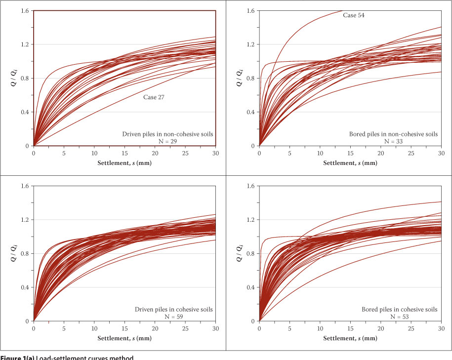
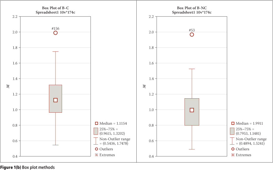
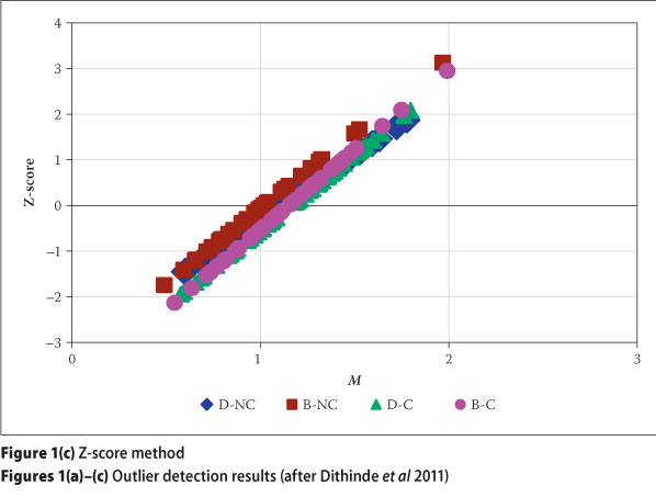
The statistical detection and treatment of outliers in the principal four sets were reported by Dithinde et al (2011). The methods used include (i) load-settlement curves, (ii) sample z-scores, (iii) box plots, and (iv) scatter plots. The results for cases with outliers are reproduced in Figure 1. Inspection of Figure 1(a) reveals two potential outliers (i.e. cases 27 and 54). The curves for these two cases depict different behaviour from the rest of the curves (case 27 with a soft initial response and case 54 with a large normalised capacity). Visual inspection of Figure 1(b) for outliers shows one data point marked as outlier for B-NC and B-C data sets. The tagged data points correspond to pile cases number 53 and 156. However, it should be noted that the box plot method for identifying outliers has shortcomings, particularly for small sample sizes as is the case here. Accordingly the identified cases will have to be corroborated by other methods. Examination of Figure 1(c) shows two data points with z-score values at a considerable distance from the rest of the data points. These data points belong to B-NC (case 53) and B-C (case 156) with z-scores of 3.13 and 2.95 respectively. Although the z-score for case 156 is less than the criterion limit value of 3, and therefore technically is not an outlier, it is sufficiently close to the limit to require further scrutiny. The results of the scatter plots of pile capacity (Q_i) versus the predicted capacity (Qp) revealed the same outliers detected by the other methods.

Aggregate of outliers

A total of five observations were detected as potential outliers, namely cases 27, 53, 54, 55 and 156. However, it is not proper to automatically delete a data point once it has been identified as an outlier through statistical methods (Robinson et al 2005). Since an outlier may still represent a true observation, it should only be rejected on the basis of evidence of improper sampling or error. Accordingly the five data points identified as outliers were carefully examined by double-checking the processes of determination of interpreted capacities and computation of predicted capacities. This entailed going back to the original data (pile testing records and derivation of soil design parameters) and checking for recording and computational errors. Following this procedure the corrections were as follows:

■ Cases 53, 54 and 55: Examination of records for these cases showed that an uncommon pile installation practice was employed. The steel piles were installed in predrilled holes and then grouted. The strength of the grout surrounding the piles contributed to the high resistance and hence the higher interpreted capacities. Since the installation procedure for these piles deviates from the normal practice, they represent a different population. These were the only piles in the database constructed in this rather unusual method. These data points were therefore regarded as genuine outliers and were deleted from the data set.

■ Case 27: There was no obvious physical explanation for the behaviour of pile case 27. The depicted behaviour is attributed to extreme values of the hyperbolic parameters representing the non-linear behaviour of the test results. Since piles in terms of pile type, size and soils conditions (i.e. cases 28 and 29) did not show similar characteristics, it was concluded that an error was made during the execution of the pile test. Accordingly this pile case was regarded as having incomplete information, and was therefore deleted.

■ Case 156: Again there was no obvious physical explanation for the behaviour of this pile case. Furthermore, the location of this data point on the scatter plot of Qi versus Qp fits the general trend for the dataset. Therefore no correction was justified for this pile case.

In summary, four outliers were removed and one retained, bringing the dataset to n = 170 cases in total and for the respective subsets ⁿD-NC = ^{28; n}B-NC = ^{30; n}D-C = ^{59; n}B-C = ^53.

 

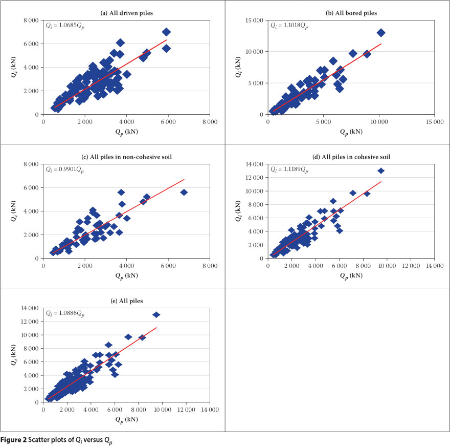
SCATTER PLOTS OF Q_I VS Q_P

Scatter plots of Q_i versus Q_p can serve as a multivariate approach to outlier detection. However they are presented here to provide an indication of whether the variance of the data set is constant or varies with the dependent variable (i.e. homoscedasticity). The ensuing scatter plots are presented in Figure 2. Visual inspection of the scatter plots seems to suggest variation in the degree of scatter increases with values of Qp. In this regard, it is evident that there is reduced scatter at smaller values of Qp. However, due to the small sample size, the case for large values of Q_p is not sufficiently clear to make any firm conclusion. Furthermore, Figure 2 gives the impression that the variance of the points around the fitted line increases linearly, thereby suggesting that the standard deviation increases with the square root of the values of Qp. This explains why the scatter tends to flatten off for large values of Q_p. The foregoing assumption implies that weighted regression analysis must be used to establish the relationship between Q_i and Qp. Such regression analysis was applied in this study (Figure 2) with the regression line forced to pass through the origin. In this case, the slope of the regression line is an estimate of the model factor M.

 

SUMMARY STATISTICS

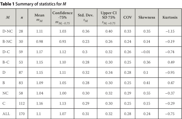
Following the outlier detection and removal process, the descriptive statistics for M consisting of mean (m_M), standard deviation (s_M), skewness and kurtosis are presented in Table 1. The sample descriptive statistics were computed using conventional statistical analysis approach. These are quantities used to describe the salient features of the sample and are required for calculations, statistical testing, and inferring the population parameters.

The sample mean m_M indicates the average ratio of Qi to Qp, with m_M > 1 indicating a conservative bias of Qi exceeding Qp. This is generally the case, with a positive bias of between 1.04 and 1.17 shown in Table 1, except for the B-NC case where Q_i is on average slightly less than Q_p with m_M = 0.98, which is slightly un-conservative. The general conservative bias reflected by m_M is, however, small in comparison to the dispersion of M as reflected by the sample standard deviation S_m for which values range from 0.23 to 0.36; the dispersion is also presented in normalised form as the coefficient of variation V_M = s_M/m_M.

The combined effect of values of m_m close to 1 and the relatively large values of S_m or V_m indicate large probabilities of realisations of M in the un-conservative range M < 1. The lower tail of the distribution of M derived from the dataset and M statistics is therefore of specific interest for application of the results in reliability assessment.

A comparison of the standard deviations or coefficient of variations for the respective cases indicates small differences. However, there seems to be a distinct trend that is influenced by the pile installation method (i.e. driven or bored). In this regard, driven piles depict higher variability compared to bored piles, irrespective of soil type. This implies that the densification of the soil surrounding the pile emanating from the pile driving process is not well captured in the selection of the soil design parameters. Even the bias for the driven piles dataset is relatively higher, thereby reiterating the notion that current practice is conservative in selecting design parameters for driven piles. Furthermore, the variability in non-cohesive materials is higher than that in cohesive materials. This is attributed to the fact that in cohesive materials the un-drained shear strength derived from the SPT measurement is directly used in the computation of pile capacity, while in non-cohesive materials, the angle of friction obtained from the SPT measurement is not directly used. Instead, the key pile design parameters in the form of bearing capacity factor (N_q), earth pressure coefficient (k_s) and pile-soil interface friction (δ) are obtained from the derived angle of friction on the basis of empirical correlation, thus introducing some additional uncertainties.

Skewness provides an indication of the symmetry of the dataset. The skewness represented in Table 1 is generally positive, indicating a shift towards the upper tail (conservative) of the values for M. There is, however, no consistent trend amongst the values for the respective datasets. The value of 0.24 for the combined dataset (ALL) could therefore be taken as indicative of the general trend. As a guideline it should be noted that the skewness of the symmetrical normal distribution is 0; for a lognormal distribution it is dependent on the distribution parameters, with a value of 0.83 based on the parameter values for the combined dataset.

Values of kurtosis indicate the peakedness of the data, with a positive value indicating a high peak, and a negative value indicating a flat distribution of the data. Negative values generally listed in Table 1 indicate flat distribution of the data, particularly for driven piles. Since these characteristics can only be captured by advanced probability distributions not generally considered in reliability modelling, kurtosis is not further considered.

In order to provide for uncertainties in parameter estimation, Table 1 also presents the confidence limits of the mean and standard deviation at a confidence level of 0.75; this is the confidence level recommended by EN1990:2002 for parameter estimation for reliability models with vague information on prior distributions. The lower confidence limit of the mean (m_m; -0.75) and the upper confidence limit of the standard deviation (s_m- +0 75) is used to present conservative estimates of the range of parameter estimates.

 

CORRELATION WITH PILE DESIGN PARAMETERS

Although the mean and standard deviation values presented in Table 1 provide a useful data summary, they combine data in ways that mask information on trends in the data. If there is a strong correlation between M and some pile design parameters (pile length, pile diameter and soil properties), then part of its total variability presented in Table 1 is explained by these design parameters. The presence of correlation between M and deterministic variations in the database would indicate that:

■ The classical static formula method does not fully take the effects of the parameter into account.

■ The assumption that M is a random variable is not valid.

Reliability-based design is based on the assumption of randomness of the basic variables. Since the model factor is among the variables that serve as input into reliability analysis of pile foundations, it is critical to verify that it is indeed a random variable. This was partially verified by investigating the presence or absence of correlation with various pile design parameters. The measure of the degree of association between variables is the correlation coefficient. The basic and most widely used type of correlation coefficient is Pearson r, also known as linear or product-moment correlations. The correlation can be negative or positive. When it is positive, the dependent variable tends to increase as the independent variable increases; when it is negative, the dependent variable tends to decrease as the independent variable increases. The numerical value of r lies between the limits -1 and +1. A high absolute value of r indicates a high degree of association, whereas a small absolute value indicates a small degree of association. When the absolute value is 1, the relationship is said to be perfect and when it is zero, the variables are independent. For the numerical correlation values in-between the limits a critical question is, "When is the numerical value of the correlation coefficient considered significant?" Several authors in various fields have suggested guidelines for the interpretation of the correlation coefficient. For the purposes of this study an interpretation by Franzblau (1958) is adopted as follows:

■ Range of r: 0 to ±0.2 - indicates no or negligible correlation

■ Range r: ±0.2 to ±0.4 - indicates a low degree of correlation

■ Range r: ±0.4 to ±0.6 - indicates a moderate degree of correlation

■ Range r: ±0.6 to ±0.8 - indicates a marked degree of correlation

■ Range r: ±0.8 to ±1 - indicates a high correlation

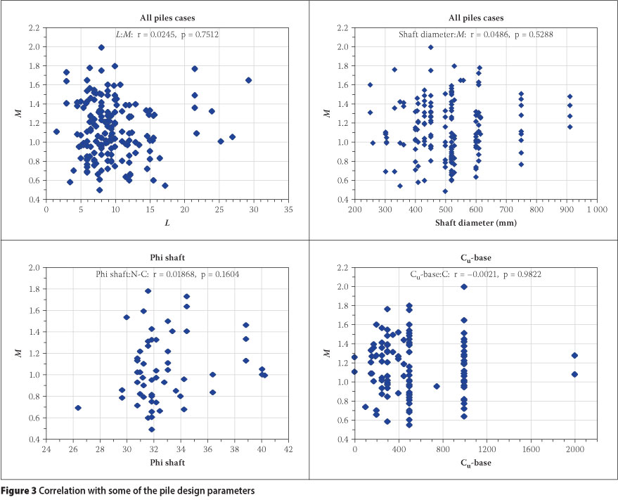
The statistical significance of the correlation is determined through hypothesis testing and presented in terms of a p-value. In this regard, the null hypothesis is that there is no correlation between M and the given design parameter (indicative of statistical independence). A small p-value (p < 0.05) indicates that the null hypothesis is not valid and should be rejected. Values for the correlation between M and the respective pile design parameters with the associated p-values are listed in Table 2. The results indicate that R < 0.4 for all the pile design parameters and therefore the degree of correlation is low. The associated p-values are generally much greater than 0.05, confirming that the correlation between the model factor and the various pile design parameters is statistically insignificant. Therefore, variations in the model factor are at least not explainable by systematic variations in the key pile design parameters, and a random variable model appears reasonable.

 

 

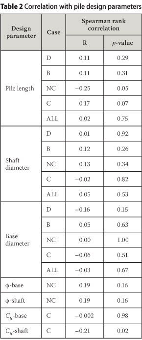
For visual appreciation of the correlation results in Table 2, some of scatter plots of M versus pile design parameters are shown in Figure 3.

 

PROBABILISTIC MODEL FOR THE MODEL FACTOR

The theory of reliability is based on the general principle that the basic variables (actions, material properties and geometric data) are considered as random variables having appropriate types of distribution. One of the key objectives of the statistical data analysis is to determine the most appropriate theoretical distribution function for the basic variable. This is the governing probability distribution for the random process under consideration and therefore extends beyond the available sample (i.e. the distribution of the entire population). Once the probability distribution function is known, inferences based on the known statistical properties of the distribution can be made.

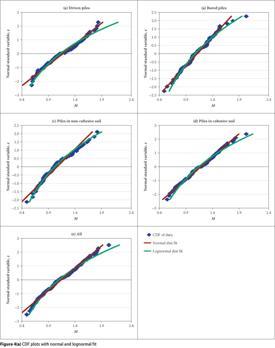
For reliability calibration and associated studies, the most commonly applied distributions to describe actions, materials properties and geometric data are the normal and log-normal distributions (Holický 2009; Allen et al 2005). Accordingly, for the current analysis only the normal and lognormal distribution fit to the data are considered. The fit is investigated through (i) a cumulative distribution function (CDF) plotted using a standard normal variate with z as the vertical axis, and (ii) direct distribution fitting to the data.

The cumulative distribution function is the most common tool for statistical characterisation of random variables used in reliability calibration (e.g. Allen et al 2005). In the context of the current analysis, the CDF is a function that represents the probability that a value of M less than or equal to a specified value will occur. This probability can be transformed to the standard normal variable (or variate), z, and plotted against M values (on x-axis) for each data point. This plotting approach is essentially the equivalent of plotting the bias values and their associated probability values on normal probability paper. An important property of a CDF plotted in this manner is that normally distributed data plot as a straight line, while lognormally distributed data on the other hand will plot as a curve. The following steps were used to create the standard normal variate plot of the CDF: ■ The capacity model factor values in a given data set were sorted in a descending order, then the probability associated with each value in the cumulative distribution was calculated as i/(n +1).

■ For the probability value calculated in Step 1 associated with each ranked capacity model factor value, z was computed in Excel as: z = NORMSINV(i/(n +1)) where i is the rank of each data point as sorted, and n is the total number of points in the data set.

■ Once the values of z have been calculated, z versus model factor (X) was plotted for each data set.

The ensuing plots are presented in Figure 4(a) from which it can be seen that the CDF for the five data sets plot more as curves than straight lines, thereby implying that the data follow a lognormal distribution. A further characterisation entailing fitting predicted normal and lognormal distributions to the CDF of the data sets is carried out. These theoretical distributions are also shown in Figure 4(a). Both distributions seem to fit the data reasonably well. However, with the exception of the bored piles data set, the lognormal distribution has a better fit to the lower tail of the data, which is important for reliability analysis and design.

To further confirm that the data best fits a lognormal distribution, z-scores are plotted as a function of Ln (M). The plots would follow a straight line if the data in fact follows the lognormal distribution. The results are presented in Figure 4(b) from which it is apparent that all the data sets plot as a straight line. This therefore confirms the strong case for a lognormal distribution assumption for the data.

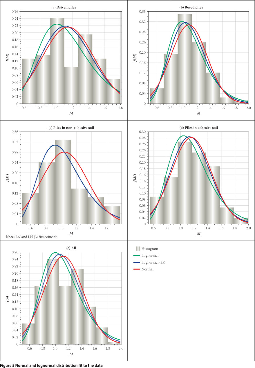
In Figure 5 the histogram of M for the respective datasets are compared to normal, lognormal and general lognormal (also three-parameter 3P) probability density function distributions based on the sample moments listed in Table 1 as distribution parameters. The graphic comparison indicates the degree to which the alternative distributions provide a reasonably smoothed representation of the M data. At the same time the approximate nature of the M data is indicated by the uneven nature of the histogram. The quantitative assessment of the difference between the empirical data frequencies and the assumed distributions is provided by the chisquare goodness-of-fit test. In this regard, the p-value is a measure of the goodness-of-fit, with larger values indicating a better fit.

In testing the hypothesis that the distribution of the data is similar to the selected probability distribution (normal or lognormal), the hypothesis is rejected if p < 0.05. The p-values for chi-square testing are presented in Table 3 from which it is apparent that such values for all the data sets are greater than 0.05 and therefore there is no evidence to reject the null hypothesis of either normal or lognormal distributions. However, on the basis of the magnitude of the p-values, the lognormal distribution seems to show a better fit compared to the other two distributions. The general lognormal distribution provides distributions which are generally intermediate between the normal and lognormal distributions (Figure 5), with similar results for the p-values (Table 3).

On the basis of the results of the two standard distribution fitting approaches studied, it can be concluded that the data fits both the normal and lognormal distributions, although the ordinary lognormal distribution has a slight edge, particularly towards the lower tail (Figure 5). However, theoretically M ranges from zero to infinity, resulting in an asymmetric distribution with a zero lower bound and an infinite upper bound. The lognormal probability density function is often the most suitable theoretical model for such data, as it is a continuous distribution with a zero lower bound and an infinite upper bound. On the basis of this practical consideration, past studies (e.g. Phoon 2005; Briaud & Tucker 1988; Ronold & Bjerager 1992; Titi & Abu-Farsakh 1999; FHWA-H1-98-032 2001; Rahman et al 2002) have recommended the lognormal distribution as the most suitable theoretical model for model uncertainty. Furthermore, in the Probabilistic Model Code by the Joint Committee on Structural Safety (JCSS) (2001), model uncertainty is modelled by the lognormal distribution. Therefore the lognormal distribution is considered a valid probability model for M. Nonetheless, it should be acknowledged that there could be some other distributions that can provide a better fit to the tails. Generally such advanced and complex distributions require a large sample size. For a small sample size, as is the case in this study, such distributions may only lead to a refinement of the results, but not a significant improvement.

 

CONCLUSIONS

Pile foundation design uncertainties are captured by the M statistics. The M statistics constitute the main input into reliability calibration and associated studies. Since the M statistics are derived from raw data, statistical characterisation of such data is of paramount importance. Accordingly characterisation of the data collected for pile foundation reliability studies have been presented in this paper. The key conclusions reached are as follows:

■ Based on the mean values for M, the static formula yields a positive bias of between 1.04 and 1.17, except for the B-NC data set where Qi is on average slightly less than Qp with mm = 0.98, which is slightly un-conservative.

■ There is a distinct trend that driven piles depict higher variability compared to bored piles, irrespective of materials type. This suggests that the densification induced by pile driving is not fully captured by existing procedures for selecting design parameters.

■ The variability in non-cohesive materials is higher than that in cohesive materials. This is attributed to the high degree of empiricism associated with the selection of pile design parameters (N_q, k_s and δ) in non-cohesive soils.

■ The values of m_M close to 1 and the relatively large values of S_m or V_m indicate large probabilities of realisations of M in the un-conservative range M < 1. Therefore the lower tail of the distribution of M is of specific interest for application of the results in reliability assessment.

■ At the customary 5% confidence level, the chi-square goodness-of-fit test results indicate that both the normal and log-normal distributions are valid theoretical distributions for M. However, when taking into account other practical considerations, the lognormal distribution is considered to be the most appropriate distribution for M.

■ None of the pile design parameters is significantly correlated with the model factor. From the probabilistic perspective, this implies that the variation in the model factor is not caused by the variations in the key pile design parameters. Therefore it is correct to model the model factor as a random variable.

 

REFERENCES

Allen, T M, Nowak, A S & Bathurst, R J 2005. Calibration to determine load and resistance factors for geotechnical and structural design. Washington DC: Transport Research Board.         [ Links ]

Briaud, J L & Tucker, L M 1988. Measured and predicted response of 98 piles. Journal of Geotechnical Engineering, 114(9): 984-1001.         [ Links ] Chin, F K 1970. Estimation of the ultimate load of piles not carried to failure. Proceedings, 2nd Southern Asian Conference on Soil Engineering, 81-90.         [ Links ]

Davison, M T 1972. High-capacity piles. ProceedingS, Soil Mechanics Lecture Series on Innovation in Foundation Construction, Chicago, American Society of Civil Engineers, Illinois Section, 22 March, 81-112.         [ Links ]

Dithinde, M 2007. Characterisation of model uncertainty for reliability-based design of pile foundations. PhD Thesis, Stellenbosch, South Africa: University of Stellenbosch.         [ Links ]

Dithinde, M, Phoon, K K, De Wet, M & Retief J V 2011. Characterisation of model uncertainty in the static pile design formula. Journal of Geotechnical and Geoenvironmental Engineering, ASCE, 137(1): 333-342.         [ Links ]

European Committee for Standardization 1997. EN-1997:2004. Eurocode 7: Geotechnical Design. Part 1: General Rules. Brussels: European Committee for Standardization (CEN).         [ Links ]

FHWA (US Federal Highway Administration) 2001. Load and Resistance Factor Design (LRFD) for Highway Bridge Substructures. Publication No FHWA-HI-98-032, Washington DC: FHWA        [ Links ]

Franzblau, A 1958. A Primer for Statistics for Non-Statisticians. New York: Harcourt Brace & World.         [ Links ]

Holický, M 2009. Reliability Analysis for Structural Design. Stellenbosch: SUN MeDIA Press.         [ Links ]

JCSS (Joint Committee on Structural Safety) PMC 2001. Probabilistic model code. JCSS Working Materials [Online] http://www.jcss.ethz.ch (retrieved 1 Feb. 2011).         [ Links ]

McBean, E A & Rovers, F A 1998. Statistical Procedures for Analysis of Environmental Monitory Data and Risk Assessment. Upper Saddle River, New Jersey: Prentice-Hall.         [ Links ]

Phoon, K K & Kulhawy, F H 2005. Characterisation of model uncertainty for laterally loaded rigid drilled shaft. Geotechnique, 55(1): 45-54.         [ Links ]

Phoon, K K 2005. Reliability-based design incorporating model uncertainties. Proceedings, 3rd International Conference on Geotechnical Engineering combined with the 9th Yearly Meeting of the Indonesian Society for Geotechnical Engineering, 191-203.         [ Links ]

Rahman, M S, Gabr, M A, Sarica, R Z & Hossan, M S 2002. Load and resistance factors design for analysis/ design of piles axial capacities. North Carolina State University.         [ Links ]

Retief, J V & Dithinde, M 2013. Pile design practice in southern Africa. Part 2: Implicit reliability of existing practice. Journal of the South African Institution of Civil Engineering, 55(1): 72-79.         [ Links ]

Robinson, R B, Cox, C D & Odom, K 2005. Identifying outliers in correlated water quality data. Journal of Environmental Engineering, 131(4): 651-657.         [ Links ]

Ronold, K O & Bjerager, P 1992. Model uncertainty representation in geotechnical reliability Analysis. Journal of Geotechnical Engineering, ASCE, 118(3): 363-376.         [ Links ]

SANS 2011. SANS 10160-5:2011: Basis of Structural Design and Actions for Buildings and Industrial Structures. Part 5: Basis for Geotechnical Design and Actions. Pretoria: South African Bureau of Standards.         [ Links ]

Titi, H H & Abu-Farsakh, M Y 1999. Evaluation of bearing capacity of piles from cone penetration test data. Project No. 98-3GT, Baton Rouge: Louisiana Transportation Research Centre.         [ Links ]

 

 

Contact details:
Dr Mahongo Dithinde
Departmert of Civil Ergireerirg
Stellerbosch University
Private Bag XI
Matielard
7602
South Africa
Departmert of Civil Ergireerirg
University of Botswana
Private Bag UB 0061
Gaberore
Botswana
T: +267 355 4297
F: +267 395 2309
E: dithirde@mopipi.ub.bw

 

Contact details:
Prof Johan Retief
Departmert of Civil Ergireerirg
Stellerbosch University
Private Bag X1
Matielard
Stellerbosch
7602
T: +27 21 808 4442
F: +27 21 808 4947
E: jvr@sur.ac.za

 

 

 

DR MAHONGO DITHINDE (Visitor) holds a PhD in Civil Engineering from the Stellenbosch University, an MSc in Foundation Engineering from the University of Birmingham (UK), and BEng in Civil Engineering from the University of Botswana. He works as a Senior Lecturer at the University of Botswana. His specialisation and research interests are in the broad area of geotechnical reliability-based design. In addition to academic work, he is also a geotechnical partner for Mattra International where he is active in consultancy work in the field of geotechnical engineering.

 

 

PROF JOHAN RETIEF (Fellow of SAICE) has, since his retirement as Professor in Structural Engineering, maintained involvement at the Stellenbosch University, supervising graduate students in the fi eld of risk and reliability in civil engineering. He is involved in various standards committees, serving as the South African representative to ISO TC98 (basis of structural design and actions on structures). He holds a BSc (cum laude) and a DSc from the University of Pretoria, a DIC from Imperial College London, and an MPhil from London University. Following a career at the Atomic Energy Corporation, he joined Stellenbosch University in 1990.