TECHNICAL PAPER

 

A model for the drying shrinkage of South African concretes

 

 

P C Gaylard; Y Ballim; L P Fatti

Contact details

 

 

---

ABSTRACT

This paper presents a model for the drying shrinkage of South African concretes, developed from laboratory data generated over the last 30 years. The model, referred to as the WITS model, is aimed at identifying the material variables that are the most important predictors of both the magnitude and rate of concrete shrinkage. In comparison with several shrinkage models already in use in the South African concrete industry, namely the SANS 10100-1, ACI 209R-92, RILEM B3, CEB MC90-99 and GL2000 models, the WITS model exhibited the best performance across a range of goodness-of-fit criteria. The ACI 209R-92 model and the RILEM B3 model showed reasonably good prediction. However, since the B3 model could be used to predict just over two-thirds of the data set, it was thus arguably the best alternative to the WITS model for the South African data set. The SANS 10100-1 model performed poorly in its predictive ability at early drying times. This may indicate that its 30-year predictions are more suited to the South African data set than its six-month predictions.

Keywords: concrete; shrinkage, model prediction, dataset

---

 

 

INTRODUCTION

Shrinkage is an important property of concrete as it influences the durability, aesthetics and long-term serviceability of the concrete, as well as its load-bearing capacity (Addis & Owens 2005). Thus, the accurate prediction of shrinkage is important in the design stage of any concrete structure (American Concrete Institute 2008). Most existing shrinkage prediction models do not take into account the effect of concrete raw materials, such as different supplementary cementitious materials and aggregate types. Furthermore, these models were generally developed using data derived from non-South African concretes and thus do not take into account the effects of local materials, which may differ substantially from those used elsewhere.

This paper presents a hierarchical, non-linear model for predicting the drying shrinkage of concrete intended for structural use. Using historical data for shrinkage of South African concretes, the model was developed by firstly identifying the most appropriate nonlinear shrinkage-time growth curve for individual shrinkage profiles. Secondly, the parameters of this growth curve model were fitted to each measured shrinkage profile individually, in terms of suitable known covariates (independent variables), namely, the composition of the concrete, its other engineering properties, as well as shrinkage test conditions. The model, referred to as the WITS model, is therefore intended to account for the raw materials used to make the concrete, the composition of the concrete (expressed through both the mixture design and the measured engineering properties of the hardened concrete), and lastly, the environmental conditions of exposure when shrinkage occurred. With reference to the database of measured shrinkage on South African concretes that was gathered for this project, the WITS model was compared to several shrinkage models that are already in use in the concrete industry.

The importance of the study is two-fold: This is the first comprehensive model to bring together laboratory data on the shrinkage of concrete generated in South Africa over a span of around 30 years, identifying the covariates which are the most important contributors to both the magnitude and rate of concrete shrinkage. Secondly, the concept of hierarchical nonlinear modelling (Davidian & Giltinan 1995), as briefly outlined above, has been applied for the first time to the modelling of concrete shrinkage. This approach could prove useful to other researchers seeking to model concrete shrinkage and related time-dependent properties such as creep. Within the limitations of the study, particularly the use of historical data, the model provides a starting point for further, statistically designed, tests and assessments to more fully explore the effects of the key variables.

 

DESCRIPTION OF THE MODEL

A detailed description of the data used in the study, its limitations and the mathematical development of the model is given in an associated publication (Gaylard et al 2012). A key limitation of the data set must be noted here, which is that the individual studies making up the data set were not necessarily carried out with the development of a model for shrinkage as the main aim. This has two consequences. Firstly, not all important factors affecting shrinkage were varied over sufficiently wide ranges. In fact, some factors were kept constant because they were known to have a significant effect on shrinkage, most notably the levels of environmental temperature and humidity maintained during the shrinkage tests. Secondly, not all data required for this study was recorded in some of the studies making up the data set. High levels of missing data led to certain potentially useful covariates (for example the 28-day compressive strength and elastic modulus of the concrete) being excluded for consideration as part of the model. However, a model can still be developed with these limitations in mind, and can then be enhanced by further, designed, experiments to include such factors.

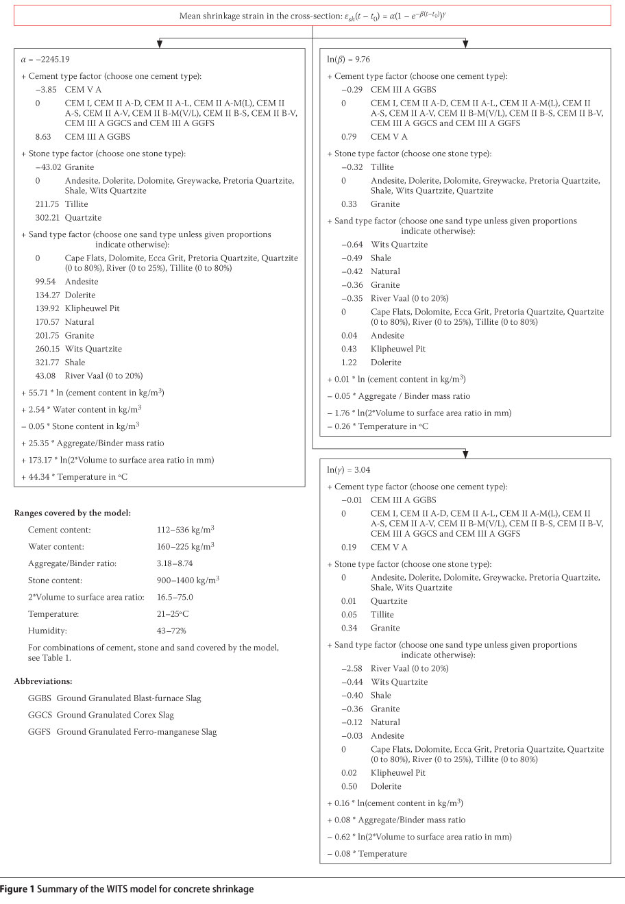
The form of the growth curve model selected is given by

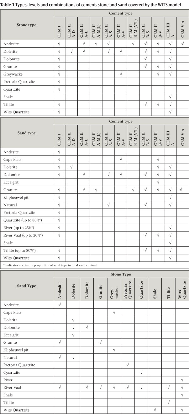
where e_sh(t - to) is the mean shrinkage strain in the cross-section (in microstrain) at drying time t - t₀ (in days) (where t is the age of the concrete and is the age at first drying in days), α represents the ultimate shrinkage (when (t - to) is very large), β represents the rate of shrinkage development with time and γ is a growth curve shape parameter which does not have a direct physical interpretation. The parameters α, β and γ in turn depend on known properties of the concrete, namely its composition, its other engineering properties and the shrinkage test conditions. The types and combinations of cement, stone and sand covered by the WITS model are given in Table 1. These are limited to the data which was available for the derivation of the model. The model parameters are given in Figure 1.

The operation of the model therefore requires that the user has to calculate the appropriate values of α, β and γ from Figure 1. These values are then substituted into Equation 1 to produce a shrinkage-time relationship for the particular concrete under consideration.

To give an indication of the fit of the model to the raw data, the two shrinkage profiles with predicted values of α closest to the observed asymptote (long-term shrinkage), as well as the two shrinkage profiles with predicted values of α furthest from the observed asymptote, from the experiments in the data set, are shown in Figure 2. The American Concrete Institute (2008) notes that the variability of shrinkage test measurements prevents models from matching measured data closely, and it is thus unrealistic to expect results from shrinkage prediction models to be within less than 20% of the test data. In this case, the two predicted profiles exhibiting the largest deviations from the raw data (Figure 2 (c) and (d)) show the last data points having deviations of 16.2% and 22.9%, respectively, which indicates that the model lies in the range of acceptable prediction.

The covariates (independent variables) which have the most significant effect on the parameters a, β and γ are listed in descending order in Table 2.

 

 

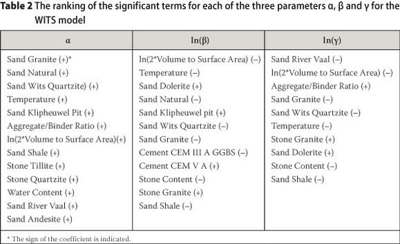
With reference to Table 2, we first consider the material parameters that influence the dependent variable a, which represents the ultimate shrinkage. The different sand types feature very strongly in the model, with three sand types (granite, natural and Wits Quartzite) making the largest contribution to high values of a. All seven sand types which were found to be significant had positive coefficients relative to the reference sand type, dolomite, which is considered to be the sand type showing the lowest shrinkage of the aggregates covered by this study (Alexander 1998). This is not an unexpected result, since a number of researchers have shown the strong influence of aggregate type on concrete shrinkage (Roper 1959; Alexander 1998; Ballim 2000). Such research indicates that this effect is due to the shrinkage of the aggregate itself, the stiffness of the aggregate and the surface characteristics of the aggregate in modifying the aggregatecement paste interface in concrete.

The next most important parameter influencing the variable α was the environmental temperature. As expected, a higher temperature leads to a higher ultimate shrinkage. The effect of the aggregate-binder ratio may be understood in terms of the restraining effect of the aggregate volume (Alexander & Mindess 2005). The specimen size effect (as represented by the ratio of the volume to the surface area of the specimen) is unexpected: the positive sign of the coefficient suggests that specimens with a lower surface area available for moisture loss, relative to their volume, are expected to reach higher levels of ultimate shrinkage. It must be noted that this variable was subject to some multi-collinearity (mostly with sand type dolerite and temperature) and thus the meaning of the magnitude and sign of the coefficient should not be over-interpreted (Gaylard et al 2012). This is certainly an aspect requiring further investigation.

The two stone types which were found to have a significant effect on α had positive coefficients relative to the reference stone type, andesite. Given the range of stone types for which sufficient data was available, andesite stone concretes showed the lowest shrinkage, and andesite was therefore used as the reference stone. Finally, the water content of the concrete also plays a role in influencing ultimate shrinkage. As expected, increasing the water content of the concrete mix increases the ultimate shrinkage.

Much less is known about the factors which influence the rate of shrinkage. However, the significant terms in the regression equation for ln(β), which represents the rate of shrinkage development with time, may be interpreted as follows: As expected, the specimen size effect is the strongest contributor to the rate of shrinkage development with time - specimens with a higher surface area available for moisture loss, relative to their volume, lose moisture more rapidly. The rate of shrinkage decreases with increasing temperature. This is unexpected, but is likely to be linked to the very narrow range of temperatures covered by this study (21-25°C) as a result of the near-constant laboratory conditions under which the shrinkage experiments were carried out. Sand type plays an important role in determining the rate of shrinkage. In contrast to the findings for the ultimate shrinkage, here the signs of coefficients for the different sand types are both positive and negative. A few cement types have an effect on the rate of shrinkage. Cements with high levels (36-65%) of GGBS (i.e. CEM III A) appeared to slow the rate of shrinkage. The effect was not statistically significant for comparable concretes containing Corex or Ferro-manganese slag. Cements containing both GGBS (18-30%) and fly ash (18-30%) (i.e. CEM V A) appeared to increase the rate of shrinkage. Increasing stone content decreases the rate of shrinkage, presumably due to the restraining effect of the aggregate. One stone type, granite, was found to increase the rate of shrinkage relative to the reference stone type, andesite.

The growth curve shape parameter ln(y) itself is difficult to interpret in the context of the growth curve equation, and thus its interpretation in terms of the significant covariates is even more difficult and was not attempted.

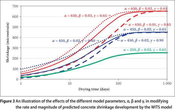
By way of illustration, Figure 3 shows a range of shrinkage profiles that are obtained with the model proposed here, using values of α, β and γ that lie within the range of values for the data set used in developing the model. Figure 3 shows the effects of the different model parameters in varying both the rate and magnitude of shrinkage development.

 

COMPARISON OF THE WITS MODEL TO OTHER PUBLISHED MODELS FOR CONCRETE SHRINKAGE

In the published literature, the most thorough model comparisons have been based on the RILEM data bank, a collection of 490 concrete shrinkage profiles mainly from North

American and European research groups (Bazant & Li 2008). The RILEM B3 model was developed on an older version of the current RILEM data bank (Bazant & Baweja 1996; Bazant 2000). In this study, model comparisons were based on the local data set, which may be considered as a smaller, South African, version of the RILEM data bank.

Five published models were used as comparisons to the WITS model developed in this study:

■ The ACI 209R-92 model developed by the American Concrete Institute (1982)

■ The RILEM B3 model developed by Bazant and co-workers (Bazant & Baweja 1996; Bazant 2000)

■ The CEB MC90-99 model developed by the Comité European du Beton (1999)

■ The GL2000 model developed by Gardner and Lockman (2001)

■ The SANS 10100-1 model adopted by the South African Bureau of Standards (2000)

■ The Eurocode 2 (EN 1992-1-1) model adopted by the European Committe for

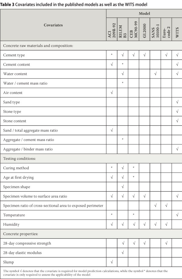
Standardization (2003). The covariates (other than drying time) used in each of these models are given in Table 3 and the ranges of applicability of each model are summarised in Table 4. The ranges of applicability of the WITS model given in Table 4 are equivalent to the ranges of the data used in fitting the model. However, the actual ranges of applicability could well be wider.

A predicted shrinkage profile was calculated for each model, including the WITS model, for each qualifying experiment in the data set (in terms of the range of applicability of each model - see Table 4), and the goodness-of-fit of these predictions to the actual data was assessed. Since the WITS model was also derived from this data set, its assessments were divided into two groups, namely the experiments used to derive the model, and the experiments which qualified to be predicted by the model but which were not used to derive the model as a result of poor quality data, for example shrinkage profiles which had not reached any indication of their long-term shrinkage value by the time measurements ceased. Combined goodness-of-fit statistics for the two groups are also presented. The ACI 209R-92, RILEM B3, CEB MC90-99 and GL2000 models were implemented according to the model specifications given in the American Concrete Institute Committee 209's guide for modelling and calculating shrinkage and creep in hardened concrete (American Concrete Institute 2008). In the ACI 209R-92 model, the air content was set at the standard value of 6%, making the air content factor equal to one, since data on this variable was not available. For the RILEM B3, CEB MC90-99, GL2000 models, 28-day cube compressive strengths were converted to the corresponding cylinder strengths using the conversion table given in the British Standard Common Rules for Buildings and Civil Engineering Structures (British Standards Institution 2004). The effective section thicknesses of most of the specimens used in the study were smaller than the minimum value of 100 mm presented in the Eurocode 2 model (European Committee for Standardization 2003). The values given in the standard were thus extrapolated to the required effective section thickness to determine the required value of the coefficient k_h:

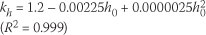
where h₀ is the effective section thickness.

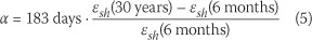
The SANS 10100-1 model was implemented according to the South African Bureau of Standards SANS 10100-1 standard (2000) for the prediction of shrinkage in concrete. The effective section thicknesses of the specimens used in this study were smaller than the minimum value of 150 mm presented in the SANS 10100-1 model. The values given in the standard were thus extrapolated to the required effective section thickness (and interpolated to the required relative humidity) by applying separate quadratic models (for the six-month and 30-year shrinkage) fitted to the shrinkage data read from the nomograph at relative humidities of 40, 50, 60, 70 and 80% and effective section thicknesses of 150, 300 and 600 mm:

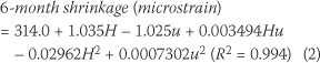
where H is the humidity in % and u is the effective section thickness in mm.

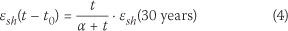
After correction for the water content of the concrete, the predicted six-month and 30-year shrinkage values were used to determine the time-shift factor, α, in the hyperbolic growth curve (Gilbert 1988; Ballim 1999) used to determine the shrinkage at other drying times:

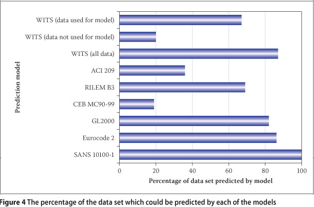
Firstly the proportion of the data set which could be predicted by a particular model was determined. This analysis is presented in Figure 4. As a result of its minimalist input requirements, the SANS 10100-1 model could be used to predict all the experiments in the data set. The WITS model had the next highest proportion of experiments which could be predicted (87%). Those experiments which did not qualify, failed to do so mostly because they used aggregate types which were not included in the derivation of the model or because of the poor quality of the shrinkage data, sometimes showing significant but unexplained deviations from the characteristic shrinkage development curve. Of this 87%, just over three-quarters of the data had been used in the development of the model, while the rest (47 experiments) had been excluded from model development because the data was insufficient to allow a realistic prediction of the ultimate shrinkage, but these experiments still qualified for prediction by the model. This latter set can thus not be regarded as a true validation data set since it comprises poor quality data compared to the overall data set. In the discussions which follow, reference to the WITS model includes consideration of all three subsets of data unless specifically indicated otherwise. The other models were able to predict lower proportions of the data set due to a combination of missing data and experiments not meeting the qualifying criteria.

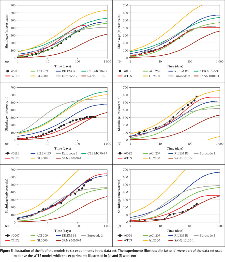
The fit of the various models to six shrinkage profiles is illustrated in Figure 5. The illustrated profiles were randomly selected from the 57 experiments to which five or all six of the models could be fitted. While the selection of the experiments was random, some effort was made to select experiments which spanned the range of shrinkage profiles in both magnitude and rate of shrinkage development. The full database containing the concrete details and shrinkage results for the 290 experiments used in this study is available at www.cnci.org.za for download at no cost.

It is clear from Figure 5 that the WITS model performed well, which was to be expected since the model was derived from the data. The SANS 10100-1 and GL2000 models tended to under- and over-predict, respectively. No particular trend regarding the performance of the other models is immediately obvious from an inspection of the results in Figure 5.

Many goodness-of-fit measures have been used by different researchers in the development of models for concrete shrinkage. The American Concrete Institute (2008) is of the opinion that "the statistical indicators available are not adequate to uniquely distinguish between models". Given this concern, it was thought best to use a broad range of these measures, both graphical and numerical, to assess the relative performance of the different models. Where possible, a critical assessment of these measures from a statistical point of view is also given.

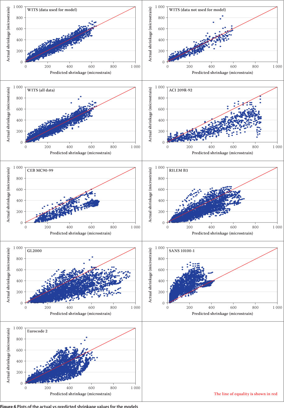
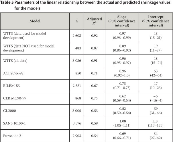
Plots of the actual versus predicted shrinkage values are shown in Figure 6. The points from an ideal model would lie entirely on the line of equality. Bazant et al (Bazant & Baweja 1995; Bazant 2000) recommend focusing on the longer drying times, where predictions are most important, since such plots are typically dominated by data gathered at short drying times. For most concrete engineering projects, designers are more concerned with long-term shrinkage. However, this is not to say that early-age shrinkage is unimportant. For example, prediction of early-age shrinkage would be very important in post-tensioned, prestressed concrete structures. The results in Figure 6 show that the WITS model, particularly at longer drying times, remained closest to the line of equality, thus indicating the best fit to the data. The adjusted R², as well as the slope and intercept, of the fitted lines to the plots are given in Table 5. A good model would have a slope close to 1 and an intercept close to 0, as well as a high adjusted R² value. The WITS model exhibited the least scatter (highest R²) and the slope closest to 1, while its intercept was the third closest to zero of all the models. This is to be expected, since a large proportion of the data was used to develop the WITS model.

Nevertheless, it is interesting to note that the international models generally over-predict the shrinkage of South African concretes. This may be related to the fact that South African concretes are generally made with crushed aggregates, resulting in a higher water demand than many northern hemisphere concretes where natural gravels are more commonly used as aggregates. On balance of the three regression criteria, the CEB MC90-99 and ACI 209R-92 models performed the next best. The over-prediction by the RILEM B3, ACI 209R-92, CEB MC90-99, Eurocode 2 and GL2000 models, as well as the under-prediction by the SANS 10100-1 model, was evident from both the plots and the regression statistics.

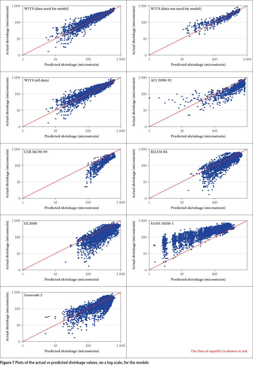
Plots of the actual versus predicted shrinkage values on a log scale are also useful since they illustrate the relative errors, which should decrease as shrinkage strain increases as a consequence of the homoscedasticity of errors (Bazant & Baweja 1995; Bazant 2000). These plots, and the parameters of their fitted lines, are shown in Figure 7 and Table 6 respectively. The WITS model was again closest to the unity line and exhibited the least scatter, indicating it to be the best model when viewed according to these criteria. The RILEM B3 model exhibited more scatter of the data around the line of equality (i.e. greater positive and negative residuals) at longer drying times than the WITS model, while the performance of the other models was worse.

In the above analysis of the results, all the concretes were allocated the same weighting. Of course, this unreasonably weights the older, lower-strength concretes, which exhibit higher levels of shrinkage strain at a given drying time. To correct for this, plots of actual versus predicted shrinkage values were both multiplied by:

where f_c28,i is the 28-day compressive strength for the experiment and f_c28,av is the average 28-day compressive strength for the data set (Bazant & Baweja 1995; Bazant 2000). This effectively normalised shrinkage according to compressive strength. However, this analysis did not change the conclusion that the WITS model performed the best, while the RILEM B3 and ACI 209R-92 models exhibited the next best performance.

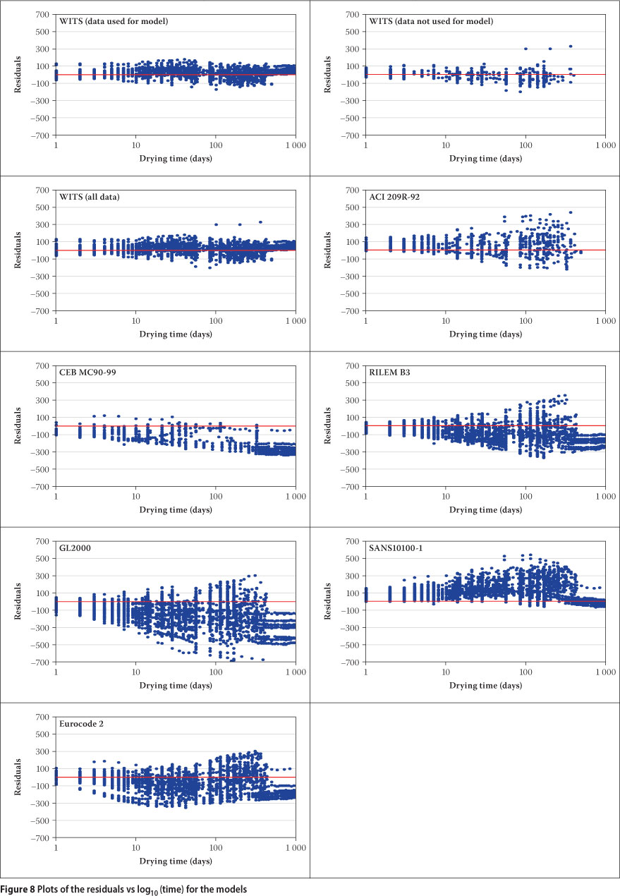
Plots of the differences between measured and predicted shrinkage (residuals) against Log₁₀(time) are shown in Figure 8. These residuals should not fan out (indicating increased deviation of a model from the raw data at longer drying times - where prediction is more important) or show any other obvious pattern or trend (McDonald &

Roper 1993, Al-Manaseer & Lam 2005). The over- and under-prediction of the different models, as discussed previously, can clearly be seen in these plots. The mean residuals for the WITS model were the closest to zero and the most consistent across the different intervals of drying time, whereas the absolute values of the mean residuals of the other models tended to increase with drying time.

The ACI 209R-92 and RILEM B3 models exhibited the next best performance on this criterion.

 

A MORE DETAILED ANALYSIS OF VARIATION

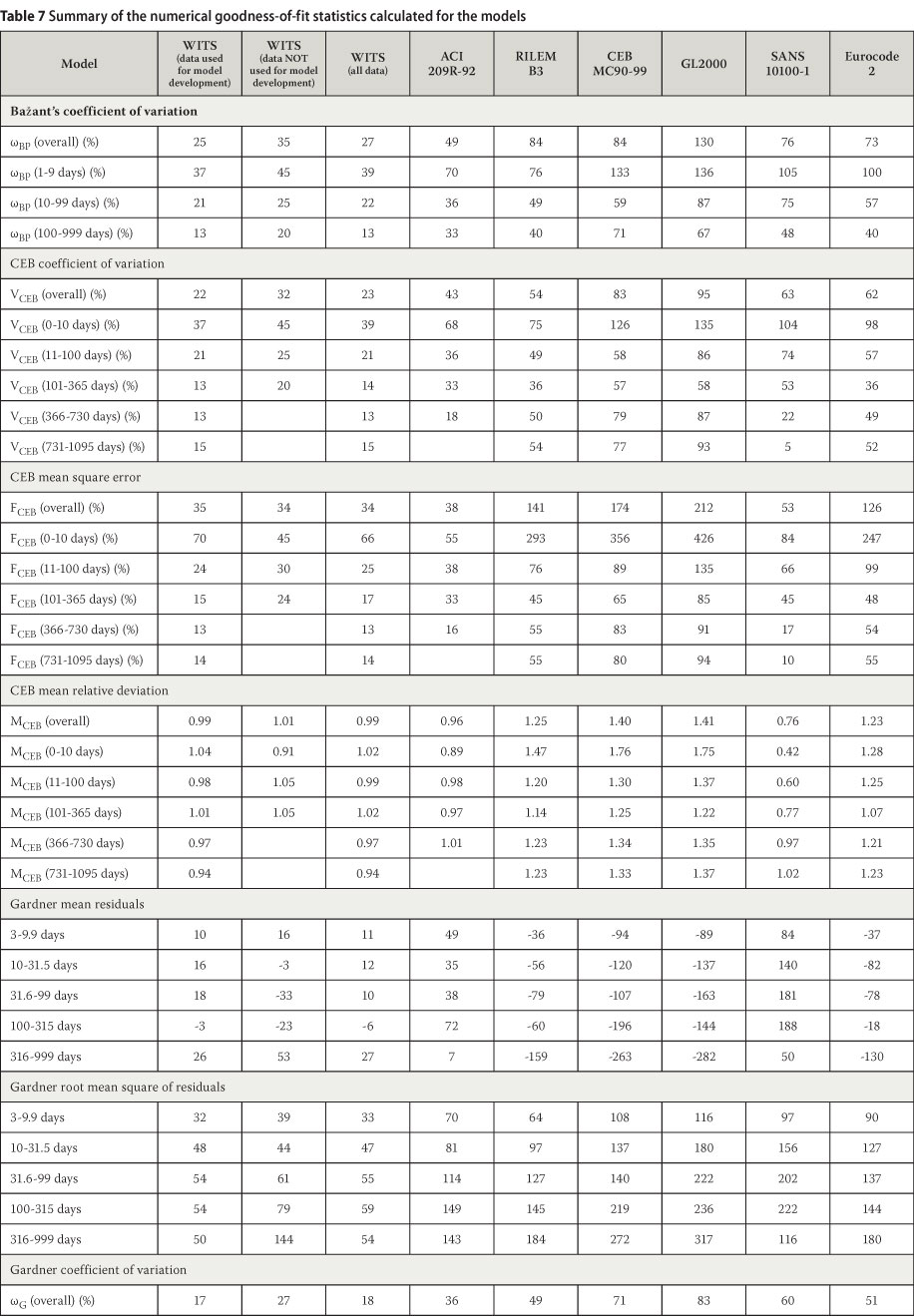
In order to further assess the suitability of the proposed WITS model, a range of numerical goodness-of-fit summary statistics were determined. Bazant's coefficient of variation, w_BP (Bazant & Baweja 1995; Bazant 2000, Al-Manaseer & Lam 2005) for all the data, as well as that calculated separately for three time intervals (on a log₁₀ scale) spanned by the shrinkage profiles, for the different models is shown in Table 7. The WITS model exhibited the lowest coefficient of variation overall, as well as across all three intervals of drying time, followed by the ACI 209R-92 model. The coefficient of variation of the WITS model, calculated on the South African data set from which the model was derived, was found to be 27%. This compares favourably to the 34% coefficient of variation for the RILEM B3 model calculated on the RILEM database, from which it was derived (Bazant 2000). This said, it should be noted that the RILEM model was developed on a larger database with a possibly greater variation in concrete types.

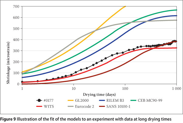
In the calculation of the CEB-FIP coefficient of variation, mean square error and mean relative deviation (Al-Manaseer & Lam 2005), all the data is pooled and then grouped into six intervals of drying time: 0-10 days, 11-100 days, 101-365 days, 366-730 days, 731-1095 days and above 1 095 days. The disadvantage of these three measures is that the data is immediately grouped into drying time intervals, which means that, although time intervals are weighted equally, different experiments are not weighted equally in the calculation of the overall mean statistics. Bazant's approach, described above, does not suffer this weakness and satisfies both these objectives. The use of the mean of the shrinkage values for a given time period rather than the grand mean of all the shrinkage values in the calculation of the CEB coefficient of variation results in large values of the coefficient of variation for short drying time intervals and vice versa. This in turn means that the calculated value of the overall coefficient of variation is unduly influenced by the short drying time data. With respect to both the Bazant and CEB coefficients of variation, it should also be noted that, for the WITS model at least, the model fit was obtained by minimising the variance, not by minimising the coefficient of variance. The use of the relative errors in the calculation of the CEB mean square error is prone to over-emphasise the errors in low shrinkage values, which are relatively less important, and vice versa. The CEB mean relative deviation is a useful statistic as it identifies the magnitude and direction of bias in the predicted values. The results from all the above calculations are given in Table 7. Results for only five time intervals are shown, since there was no data at drying times longer than 1 095 days in the data set used in this study. The WITS model exhibited the lowest overall CEB coefficient of variation, followed by the ACI 209R-92 and RILEM B3 models. Over the different time intervals, the WITS model had the lowest coefficient of variation, except for the longest drying time interval (731-1 095 days) where it was superseded by the SANS 10100-1 model. It appeared that the SANS 10100-1model is a good predictor of shrinkage at longer drying times, but under-predicts at shorter drying times, perhaps due to poor prediction of the six-month shrinkage, as illustrated in Figure 5, and also in Figure 9 for an experiment which includes data at very long drying times. The over-emphasis of the CEB mean square error statistics for low shrinkage values (and vice versa), as discussed above, can clearly be seen (Table 7). The WITS model, closely followed by the ACI 209R-92 and SANS 10100-1 models, performed better than the other models on this measure. The CEB mean relative deviation statistics are shown in Table 7, which illustrate the magnitude and direction of the bias in the different models (discussed previously), as a function of drying time. The WITS model showed the least bias across all time intervals, closely followed by the ACI 209R-92 model. The narrowing difference between the actual and predicted values of the SANS 10100-1 model with increasing drying time is shown clearly here, again indicating that the longer-term (30-year) predictions of this model are more in line with the measured data than the shorter-term (six-month) predictions.

In the method used by Gardner (2004), the observations are grouped into half-log decades (starting at a drying time of three days). Within each time interval, the average and the root mean square (RMS) values of the differences between the actual and predicted values (residuals) are calculated. The trend of the average residual with time shows whether there is over- or under-estimation (bias) with time by the model, while the trend of the RMS values with time shows if the deviation of the model increases with time. Next, the RMS values are simply averaged. The average RMS values are then normalised by dividing by the average of the average shrinkage values (for the different time intervals) to produce a measure analogous to a coefficient of variation. This formula given by Gardner is, however, incorrect, since the mean squares, not RMS values, should be averaged. In this study, the corrected formula for the Gardner coefficient of variation, w_G, was applied. As in the case for the overall CEB statistical indicator, wG also suffers from the disadvantage that the data is immediately grouped into drying time intervals, which means that, although time intervals are weighted equally, experiments are not weighted equally in the calculation of this overall mean statistic.

The Gardner average residuals and the root mean squares of the residuals for the different time periods for all the models are given in Table 7. The WITS model had the lowest mean residuals, followed by the ACI 209R-92 model. The bias towards over- or under-prediction by the other models can clearly be seen. The Gardner coefficient of variation also identified the WITS model as the best model according to this criterion, as did the root mean squares of the residuals for the different drying time intervals. The latter statistic showed that the deviations of all the models increased with time, with the exception of the WITS model (over all drying times) and the SANS 10100-1 model (at long drying times).

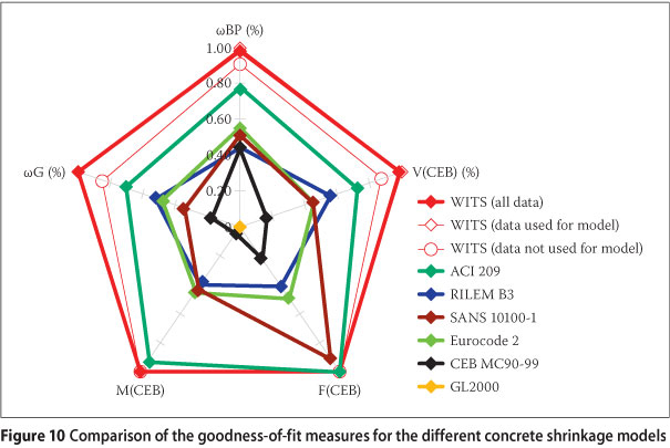
The discussion above has shown that there is no single goodness-of-fit statistic which can adequately capture all aspects of the performance of a model for the shrinkage of concrete. In order to summarise the information contained in the different overall numerical goodness-of-fit measures discussed above, their calculated values for the different models are represented in Figure 10 by means of a radar chart. This plot showed that, across all the goodness-of-fit measures, the WITS model performed the best. This was perhaps to be expected, since the model was derived largely from this data. However, even the performance of the model on the data which was not used in the development of the model was excellent, although, as was mentioned earlier, this small data set should not be regarded as a true validation data set. The ACI 209R-92 model exhibited the second-best performance, but here it must be noted that this model could be used to predict only 36% of the data set. The third best performance across the goodness-of-fit indicators was shown by the RILEM B3, SANS 10100-1 and Eurocode 2 models indicating that these are arguably the best alternative models to the WITS model for the South African data set. The SANS 10100-1 model performed poorly relative to the other models, but as discussed above, its predictive ability at longer drying times was better than that at shorter drying times. This may indicate that its 30-year predictions are more suited to the South African data set than its six-month predictions, i.e. that the time development of shrinkage of the model may need to be adjusted relative to the British Standard from which the model was directly taken.

 

CONCLUSIONS

The WITS model presented in this paper represents a first attempt at applying the concept of hierarchical nonlinear modelling to the prediction of shrinkage for South African concretes. Furthermore, this is the first time that a shrinkage model has been derived from a gathering of test data on the shrinkage of concretes which had been generated by a range of South African laboratories over a span of 30 years. The proposed model identifies the material and environmental covariates that are the most important contributors to both the magnitude and rate of concrete shrinkage. Based on a range of reliability and goodness-of-fit measures, the WITS model was found to perform better than a number of local and international models on the basis of the magnitude and rate of prediction at both early and late drying times. The coefficients proposed for the model have yet to be confirmed through further testing with a wider range of material and environmental variables. This will require further, statistically designed, shrinkage tests that are aimed at exploring the effect of key variables more fully. This approach could also prove useful to future research seeking to model concrete shrinkage and related time-dependent properties such as creep.

 

ACKNOWLEDGEMENTS

The provision of data and helpful comments by Prof Mark Alexander and Dr Hans Beushausen (Department of Civil Engineering, University of Cape Town, Cape Town, South Africa) are gratefully acknowledged. The authors are also grateful to the Cement and Concrete Institute for their data and logistical support and, together with Eskom, for their financial support to our research programme.

 

REFERENCES

Addis, B J & Owens, G (Eds) 2005. Fundamentals of Concrete. South Africa: Cement and Concrete Institute, 35-49.         [ Links ]

Al-Manaseer, A & Lam, J-P 2005. Statistical evaluation of shrinkage and creep models. ACI Materials Journal, 102(3): 170-176.         [ Links ]

Alexander, M G 1998. Role of aggregates in hardened concrete. In: Skalny, J P & Mindess, S (Eds), Materials Science of Concrete V, Westerville, OH: American Ceramic Society, 119-147.         [ Links ]

Alexander, M G & Mindess, S 2005. Aggregates in Concrete. London: Taylor & Francis.         [ Links ]

American Concrete Institute (ACI) 1982. Prediction of creep, shrinkage and temperature effects in concrete structures. In: Designing for creep and shrinkage in concrete structures, ACI 209R-82, Detroit: American Concrete Institute, 193-300.         [ Links ]

American Concrete Institute (ACI) 2008. Guide for modeling and calculating shrinkage and creep in hardened concrete. ACI 209.2R-08, Detroit: American Concrete Institute.         [ Links ]

Ballim, Y 1999. Localising international concrete models - The case of creep and shrinkage prediction. proceedings, 5th International Conference on Concrete Technology for Developing Countries, New Delhi, India, Vol III, 36-45.         [ Links ]

Ballim, Y 2000. The effects of shale in quartzite aggregate on the creep and shrinkage of concrete - A comparison with RILEM model. Materials and Structures, 33: 235-242.         [ Links ]

Bazant, Z Ρ 2000. Creep and shrinkage prediction model for analysis and design of concrete structures: Model B3. proceedings, Adam Neville Symposium: Creep and Shrinkage - Structural Design Effects, 1-84.         [ Links ]

Bazant, Z P & Baweja, S 1995. Justification and refinement of Model B3 for concrete creep and shrinkage. 1. Statistics and sensitivity. Materials and Structures, 28: 415-430.         [ Links ]

Bazant, Z P & Baweja, S 1996. Creep and shrinkage model for analysis and design of concrete structures - Model B3. Materials and Structures, 28: 357-365 (with errata in 29: 126).         [ Links ]

Bazant, Z P & Li, G-H 2008. Comprehensive database on concrete creep and shrinkage. ACI Materials Journal, 105(6): 635-637.         [ Links ] British Standards Institution 2004. BS EN 1992-1-1:2004I: Common Rules for Buildings and Civil Engineering Structures. London: British Standards Institution.         [ Links ]

Davidian, M & Giltinan, D M 1995. Nonlinear Models for Repeated Measurement Data, 1st ed. London: Chapman & Hall.         [ Links ]

European Committee for Standardization 2003. EN 1992-1-1: Eurocode 2: Design of Concrete Structures - Part 1: General Rules and Rules for Buildings. Brussels: European Committee for Standardization.         [ Links ]

Federation Internationale du Beton 1999. Structural Concrete - Textbook on Behaviour, Design and Performance. Updated Knowledge of the CEB/FIP Model Code 1990. FIB Bulletin, Vol. 2, Lausanne, Switzerland: Federation Internationale du Beton, 37-52.         [ Links ]

Gardner, N J & Lockman, M J 2001. Design provisions for drying shrinkage and creep of normal strength concrete. ACI Materials Journal, 98(2): 159-167        [ Links ]

Gardner, N J 2004. Comparison of prediction provisions for drying shrinkage and creep of normal-strength concretes. Canadian Journal of Civil Engineering, 31(5): 767-775.         [ Links ]

Gaylard, P, Fatti, L P & Ballim Y 2012. Statistical modelling of the shrinkage behaviour of South African concretes. In preparation, to be submitted to the South African Statistical Journal.         [ Links ]

Gilbert, R I 1988. Time Effects in Concrete Structures. Amsterdam: Elsevier.         [ Links ]

McDonald, D B & Roper, H 1993. Accuracy of prediction models for shrinkage of concrete. ACI Materials Journal, 90(3): 265-271.         [ Links ]

Roper, H 1959. Study of shrinking aggregates in concrete. CSIR Technical Report 502, Pretoria: Council for Scientific and Industrial Research.         [ Links ]

South African Bureau of Standards 2000. SANS 10100-1: The Structural Use of Concrete. Part 1: Design. Pretoria: South African Bureau of Standards.         [ Links ]

 

 

Contact details:
Dr Petra Gaylard
School of Statistics and Actuarial Science
University of the Witwatersrand
Private Bag 3, Wits, 2052
South Africa
T: +27 11486 4836
F: +27 86 671 9895
E: petra.g@mweb.co.za

 

Contact details:
PROF Paul Fatti
School of Civil & Environmental Engineering
University of the Witwatersrand
Private Bag 3, Wits, 2052
South Africa
T: +27 11 717 112'
F: +27 11 717 1129
E: yunus.ballim@wits.ac.za

Contact details:
Prof Paul Fatti
School of Statistics and Actuarial Science
University of the Witwaters and Private Bag 3, Wits, 2052
South Africa
T: +27 11 880 6957
F: +27 11 788 9943
E: paulfatti@gmail.com

 

DR PETRA GAYLARD holds a PhD in Chemistry and an MSc in Statistics from the University of the Witwatersrand. This publication arises from sthe research report for her MSc in Statistics.

 

 

PROF YUNUS BALLIM holds BSc (Civil Eng), MSc and PhD degrees from the University of the Witwatersrand (Wits). Between 1983 and 1989 he worked in the construction and precast concrete industries. He has been at Wits since 1989, starting as a Research Fellow in the Department of Civil Engineering and currently holds a personal professorship. He was the head of the School of Civil and Environmental Engineering from 2001 to 2005. In 2006 he was appointed as the DVC for academic aff airs at Wits. He is a Fellow of SAICE.

 

 

PROF PAUL FATTI is Emeritus Professor of Statistics at the University of the Witwatersrand and acts as consultant in Statistics and Operations Research to a broad range of industries. He holds a PhD in Mathematical Statistics from the University of the Witwatersrand and an MSc in Statistics and Operational Research from Imperial College, London. He spent most of his professional career at the University of the Witwatersrand, including 18 years as Professor of Statistics. His other employment includes the Chamber of Mines Research Laboratories, the Institute of Operational Research in London and the CSIR.