Comparison and evaluation of mathematical lactation curve functions of Iranian primiparous Holsteins

 

 

M. Elahi Torshizi^I,#; A.A. Aslamenejad^I; M.R. Nassiri^I; H. Farhangfar^II

^IDepartment of Animal Science, Faculty of Agriculture, Ferdowsi University of Mashhad, Mashahd, Iran
^IIDepartment of Animal Science, Faculty of Agriculture, Birjand University, Birjand, Iran

 

 

---

ABSTRACT

Describing lactation in mammals using a lactation curve aims to provide a concise summary of the pattern of milk yield and valuable information about the biological and economic efficiency of the animal or herd under consideration. A total of 106 581 monthly test-day milk records collected from 12 677 Tehran Province primiparous Holstein cows from 151 herds, were used in this study. Using the General Linear Model procedure in SAS, the effect of herd, calving year, age at calving, season of production, age and days in milk were found to be significant on daily milk yield. The suitability of seven mathematical models (with three, four and five parameters) for describing the 305-day milk yield lactation curve of Holstein cows, were examined in this study. Comparisons of the models were made based on the coefficient of determination, root mean square error, Durbin Watson coefficient and sum of daily deviations, by using nonlinear (NLIN), regression (REG) and autoregression (AUTOREG) procedures in SAS. The best three, four and five parameter functions with respect to these criteria were the Incomplete Gama, Dijkstra and Grossman functions. With regards to the Wilmink model, the best results obtained were from models with the constant of 0.05 and 0.065. The Wood function was selected as the best model for prediction of daily milk yield, due to parameters in the function and less computational limitation.

Keywords: Daily milk yield, goodness of fit, lactation, model comparison

---

 

 

Introduction

The graphical representation of daily milk yield against time after calving is called a lactation curve (Sherchand et al., 1995). The shape of a standard lactation curve may be described as increasing, at a relatively high rate, up to the point where peak production is obtained, after which it declines at a slower rate until the end of milk production (Lombaard, 2006).

A mathematical model of the lactation curve provides summary information about culling and milking strategies, future milk yields of an individual animal or a herd and dairy cattle production. It is useful for management and making breeding decisions and simulating a dairy enterprise (Olori et al., 1999). It has been documented that the lactation curve is influenced by environmental factors such as the herd, year of calving, parity, age and season of calving (Wood, 1967; Tekerli et al., 2000). Models to describe the lactation curve have been classified into two main groups: linear and nonlinear models. In the linear models, like the polynomial regression model (Ali & Scheaffer, 1987) or the mixed log model (Guo & Swalve, 1995), parameters are linear functions of days in lactation or transformation thereof, and can be computed by simple linear regression. Nonlinear models such as the Incomplete Gamma function (Wood, 1967) or Wilmink function (Wilmink, 1987), need iterative techniques to be solved (Vargas et al., 2000). Different iterative methods frequently employed in nonlinear regression models are Marquardt, Newton, Gauss and Dud. During the last decade, several mathematical models have been developed to describe the shape of the lactation curves (Wood, 1967; Ali & Schaeffer, 1987; Wilmink, 1987; Grossman et al., 1988; Rook et al., 1993; Guo & Swalve, 1995; Dijkstra et al., 1997). Rowlands et al. (1982) reported that Wood's curve does not provide a consistently good fit to data of high producing dairy cows in the peak of milk production. Ali & Schaeffer (1987) reported that a regression model for milk yields on day in lactation (linear and quadratic) and on the log of 305-d divided by day in lactation (linear and quadratic) were better than the Gamma function. A study of lactation curves in dairy cattle on farms in central Mexico showed that the Dijkstra function was superior to the Wood, Wilmink and Rook functions for describing the lactation curve (Val-Arreola et al., 2004). Dag et al. (2005) showed that the cubic model compared to the Wood, inverse polynomial and quadratic functions made the best fit and described the shape of the lactation curve of Awassi ewes well and therefore the correlation coefficient was highest between total milk yield and estimated milk yield for this model. Comparison of different functions showed that the best fit was for the Ali & Schaeffer function (Olori et al., 1999). However, it was only slightly better than that of Wilmink. Parameter k of the Wilmink curve is associated with the time of lactation peak and this implies that the Wilmink model had three parameters. Other studies used different constant k parameters i.e. 0.05, 0.065 and 0.10 (Wilmink, 1987; Macciotta & Vicario 2005; Silvestre et al. 2006). Dag et al. (2005) demonstrated that the cubic model made the best fit to the data collected from Awassi ewes and allowed a suitable description of the shape of the lactation curve.

The objectives of this study were to asses some of the environmental factors affecting daily milk yield (DMY) to compare the goodness of fit of mathematical (linear and nonlinear) functions of the lactation curve separately as well as evaluation of nonlinear models with respect to the number of parameters. Also the Wilmink function using different k constants (0.05, 0.10, 0.61, and 0.065) were evaluated.

 

Materials and Methods

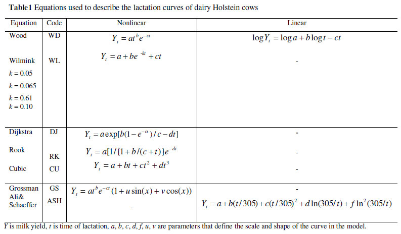
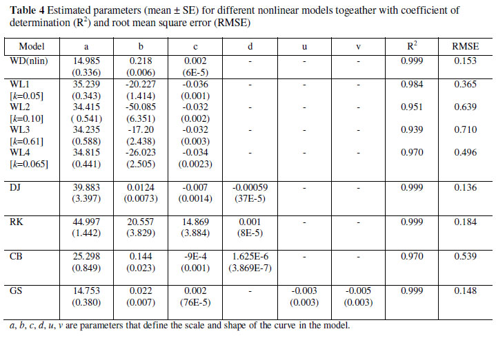
The initial dataset consisted of 257 846 first lactation test-day records of primiparous Holstein cows from the Tehran Province of Iran. All cows had three times a day milking. The data were edited based on the following criteria: a) lactation period should be between 200 and 305 days; b) the number of test-day records for each lactation should be at least 5; c) age at calving should be between 18 and 29 months and was classified into 12 classes and d) individual daily milk production should be between 3 and 85 kg. The final dataset included information of 106 581 monthly test-day records. Seven different models were selected from the literature and analysed in this study (Table 1). The Wood model (WD) was tested in two different forms i.e. nonlinear and linear. The nonlinear form was linearized by taking the natural logarithm from each side of the equation because nonlinear regression does not guarantee convergence (Ruiz et al., 2000). The Wood model is a gamma function, in which a approximates the initial milk yields after calving, b is the inclining slope parameter up to yield peak, and c is the declining slope parameter (Wood, 1967).

Wilmink (1987) introduced two lactation models. In the first model, a quadratic term was added and an adjustment made to the exponential term. This model (WL) was then adjusted to obtain the second model by dropping the quadratic term from the initial function. In this model a is the level of production, b is the initial raise to peak and c is the decreasing rate after peak. The factor k was set equal to 0.05 and is associated to the time of peak yield. Olori et al. (1999) estimated this factor to be 0.61, while (Brotherstone et al., 2000) assumed the constant parameter to be 0.10 and in preliminary analysis, it was estimated to be 0.065 (Silvestre et al. 2006). The other model was the Dijkstra model (Dijkstra et al., 1997) which is a mechanistic model with four parameters that describes the mammary growth pattern (cell proliferation and apoptosis) of mammals during pregnancy and lactation (DJ).

Rook et al. (1993) proposed a four parameter model (RK) and attempted to model lactation as the product of a constant, a, a monotonically increasing function of time, <1(t) , and a monotonically decreasing function of time <2(t). The Grossman model (GS) was also used in this study. It is a modified form of the Wood's model by including sinus and cosinus terms to account for seasonal variations (Grossman & Koops, 1988). In this model v is the coefficient of calving season and u is coefficient of year of the considered as measured radian (Kocak & Ekiz, 2008).

The cubic model (CU) and Ali & Schaeffer (ASH) models were the other functions used to describe the lactation curve in this study. The ASH model was a regression model of yields on day in lactation (linear and quadratic) and log of 305-day yield divided by day in lactation (linear and quadratic) fitted.

Proc NLIN, REG and AUTOREG in SAS (2005) were employed to fit the nonlinear and linear regression functions. Factors affecting test-day milk yield of cows were evaluated by using the general linear model procedure (PROC GLM) of SAS (2005). Results were given as least-square means (LSM) of daily milk yield (DMY) with standard errors. When nonlinear functions were fitted, the Gauss-Newton method was used as the iteration method.

The goodness of fit the models was evaluated using the following criteria:

• R²- Coefficient of determination which equals the percentage of variance of monthly yields explained by the model:

where SSE is error sum of square and SST is total sum of square.

• RMSE-Root mean square error which is a kind of generalized standard deviation:

where n is the number of observations, yi are the actual values and ŷ are values predicted by the regression model. Smaller RMSE indicates better modelling.

• AIC-Akaike's Information criterion: AIC is a measure of the goodness of fit of an estimated statistical model (Akaike, 1974). It can describe the tradeoff between bias and variance in model construction. AIC is not a test on the model in the sense of hypothesis testing; rather it is a tool for Model selection. Given a data set, several competing models could be ranked according to their AIC, with the one having the lowest AIC being the best. In the general case the AIC is:

AIC =-2 log L + 2K

where K is the number of estimated parameters in the model but L is the maximized value of the likelihood function for the estimated model.

• DW --Durbin-Watson coefficient:

where e_t is residual at time e and e_t-1 is residual at time t-1.

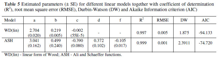
The Durbin-Watson statistic tests the null hypothesis that the residuals from an ordinary least-square regression are not autocorrelated against the alternative that the residuals follow an autoregressive process. The Durbin-Watson statistic ranges in value from 0 to 4. A value near two indicates non autocorrelation; a value toward 0 indicates positive autocorrelation; a value toward 4 indicates negative autocorrelation. AIC and DW criteria were only applied for comparison of the linear form of WD and the ASH functions in this study.

• SDD - Sum of daily deviation:

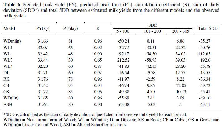
The sum of differences between predicted daily milk yield by each model and average milk yield was calculated in different stages of the lactation (5 -100 days, 101 -200 days and 201 -305 days). Positive or negative amounts of SDD show that the model overestimated and understimated milk yield in a specific period. Furthermore, predicted peak yield (PY) and predicted peak time (PT) were calculated for different models, as well as the correlation coefficient (R) between the estimated milk yields and actual milk yields in the dataset.

Linear and nonlinear functions were compared separately with these criteria, because the characteristics of these models are different.

The effect of environmental factors and covariates on milk yield parameters was investigated by analysis of variance (PROC GLM) with the following model:

where Y_nijkl is daily milk yield of n^th animal affected by i^th herd (151 herd), j^th calving year (10 years from 1999 to 2008), k^th season of milk production (four seasons: 1 -spring, 2 -summer, 3 - autumn, 4 -winter), l^st age at first calving class (12 months from 18 to 29), b_R is the linear regression coefficient of age at test (covariate), b_M is the linear and quadratic regression coefficient of days in milk (covariate) and e_nijkl is the random effect of residuals with expectation and variance equal to 0 and δ_e² respectively. µ is the overall mean, H_i, CY_j, S_k and AGC_l are effects of herd, calving year, season of milk production and age at first calving, respectively.

 

Results and Discussion

Descriptive statistics for the final data set are presented in Table 2.

 

 

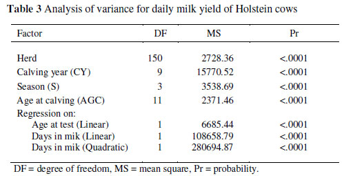
Changes in management, feeding regimen and other environmental factors are usually responsible for some of milk yield variation over years (Hatungumukama et al., 2008). The overall mean of daily milk yield for the cows in this study was 29.18 kg/d. The results of the analysis of variance are shown in Table 3. Similar factors are reported in the literature to influence milk production significantly (Jamrozik & Schaeffer, 1997; Tekerli et al., 2000; Farhangfar & Naeemipour, 2007). Differences in milk production amongst herds are due to variation in management, feeding and other environmental factors, as well as annual climatic changes. A constant increase was observed in DMY from calving years 1999 to 2008. The minimum least square means (LSM) for DMY, 24.99 ± 0.11 kg/d was observed in 1999 and it increased gradually to reach 29.67 ± 0.09 kg/d (Figure 1).

 

 

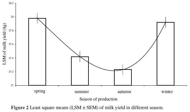
This shows that knowledge of feeding, breeding and economic management of dairy herds has improved since 1999. Least square means of daily milk yield in different seasons of production are presented in Figure 2. LSM of DMY was significantly different between the four seasons (P <0.001). The maximum LSM's of daily milk yield were observed in spring and winter (27.98 ± 0.07 kg and 27.92 ± 0.07 kg, respectively), and the minimum in summer and autumn (27.42 ± 0.07 kg and 27.23 ± 0.07 kg). The LSM of summer and autumn did not differ significantly (P >0.05). In this study, DMY was low in the dry season and the following summer season, because of low availability of natural fresh pastures and due to high temperatures during summer.

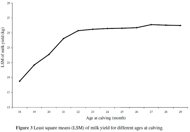
The mean age at first calving was 24.9 months. The results of this study show that LSM of DMY increased with the calving age in the first parity (Figure 3). The minimum LSM of DMY was observed for cows calving at 18 months of age (18.52 ± 0.79 kg/d). It then gradually increased up to calving at 24 months of age (25.59 ± 0.098 kg/d) after which it stayed constant. Increased milk production with increasing age at calving in the first parity is consistent with results reported by other authors (Hatungumkama et al., 2008).

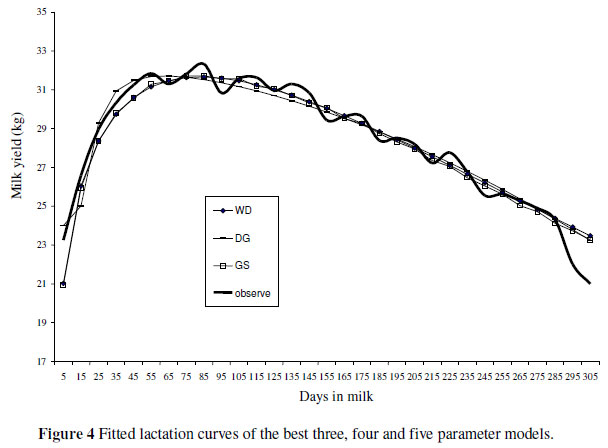
Estimated parameters and goodness of fit statistics of nonlinear models are presented in Table 4. In nonlinear models, R² ranged from 0.93 to 0.99 but in linear models, R² was almost the same (Table 5). However, RMSE of the models differed. The range of RMSE was between 0.136 and 0.710 for the nonlinear models. Amongst three parameter models (Wood & Wilmink), the Wood model was better than Wilmink models. It had the higher R² and smaller RMSE. The results for the WL models (with different constants) show that the best models were WL1 and WL4, respectively. They could predict milk yield accurately across the lactation. Figure 4 indicates that the average milk yield of the data set increased from 23.3 kg/day at day 5 of lactation to the peak yield of 32.4 kg/day on day 85 and subsequently declined to 21 kg/day on day 305.

Predicted peak times (PT) of the WD and WL models differed, with PT of the WD model (81 days) being much closer to the actual peak time compared to the WL models (30 -66 days). However, predicted peak yield (PY) of the WD model was lower (31.7 kg) than that of the WL models (32.1 -33.4 kg), which was closer to the actual peak yield of the data set. Amongst the Wilmink models, the magnitudes of peak yield were comparable, with the earliest peak time predicted by the WL3 model and the latest by the WL1 model (Table 6). WL1 and WL4 underpredicted milk production less than WD during early lactation but W3 overpredicted milk yield in this period (Table 6).

Scott et al. (1996) reported that the WD model has the tendency to overestimate milk yield prior to peak and at the final stage of lactation. Results of this study showed that the WD equation underestimated milk yield in the days 5 -100 period. The total SDD in the non-linear Wood function was lower than that of the WL models. Amongst the WL models, the WL1 showed the lowest total SDD. Furthermore, the WL models underestimate milk yield in the 101 -200 day period and overestimated it at the final stage of lactation (Table 6). The correlation between the estimated and observed milk yields was higher when using the WL1 model (0.92) compared to the WL2, WL3 and WL4 models, but it was smaller than that of the WD model. Olori et al. (1999) showed that weekly average daily milk yield was fitted best by the WL equation with k = 0.61, and worst by the WD model. The result of this study does not confirm Olori's report. The WL3 model with k = 0.61 had the smallest R² and highest RMSE compared to the WL1, WL2 and WL4 models (Table 4). Furthermore, the WL3 model did not fit the lactation curve as well as the WD equation (Table 6).

In four parameter models (DJ, RK and CB), the ranges of R² and RMSE were between 0.97 to 0.99 and 0.136 to 0.539, respectively (Table 4). In these models, peak yield was similar (around 31.5), but the CB model showed the latest estimate of PT amongst the three and four parameter models. Predicted PT for the DJ model was at 60 days, which is not close to the observed peaking time (85 days), while PT was late for the CB model (95 days) (Table 6).

The RK and CB models underestimated milk yield in the first period of lactation (5 -100 day), but the rate of deviations decreased as days in milk increased. According to the R² and RMSE the DJ model was the best of all these models. Val-Arreola et al. (2004) also reported that the DJ equation was the best option to be used in describing the lactation curve. The DJ equation is the best four parameters equation, because it is a mechanistic model that represents biological interpretation for the parameters. The most desirable model would be one with a limited number of parameters and a biological interpretation (Rekaya et al., 2000). In general, goodness of fit of the DJ equation was better than that of the WD model (with respect to SDD and biological interpretation). Both of these models had similar R², but RMSE of the DJ model was smaller than that of the WD model. Comparison with WL1 showed that these models fit the lactation curve more accurately. With respect to the number of parameters, it can be concluded that the best three and four parameter models are WD and DJ, respectively (Figure 4, Tables 4 and 6). This is in agreement with results of Val-Arreola et al. (2004) that showed the DJ equation was the best option for describing lactation curves in central Mexican dairy cows. They mentioned that the WD equation explained much of the variation, but its parameters did not have direct biological interpretation. Therefore, it seems that this characteristic (the number of parameters) was not important for their study.

Evalution of the RK and CB models showed that estimated PT of the RK model (78 days) was earlier than that of the CB model (95 days). PY of both models were almost the same while total SDD of the RK model was lower than that of the CB model. In general, the RK equation gave a similar goodness of fit as the WD (nlin) model, but RMSE was lower for the WD model and PT was nearer to the actual peak yield compared to that of the RK model. Therefore, the WD model fitted the data better compared to the RK model.

Evaluation of the GS model (with five parameters) showed that its R² is as good as that of the WD model (Table 5). The reason for this equality might be due to the more parameters of this model compared to that of the WD model. The PY of the GS model was 31.7 kg and PT was on day 85, which were similar to that of the observed data. Regardless of the number of parameters, the GS model was one of the best five parameter models to describe monthly milk yield recordings. In the study of Soysal & Gurcan (2000) who compared the Wood, Goodall and Grossman models, the highest R² value was reported for the Grossman model.

Estimated parameters for the differenct linear models (WD and ASH), are presented in Table 5. As shown in this table, the coefficient of determination of the ASH model was slightly better than that of the WD model and the RMSE was lower. The Durbin-Watson statistics show that the WD and ASH equations have positive and negative auto-correlation of residuals, respectively.

Positive autocorrelation occurs when adjacent values of residuals tend to share the same sight (positive or negative) more than randomly possible (Dematawewa et al., 2007). Furthermore, the AIC statistic for the WD was better than that of the ASH model. Predicted PY and PT for both of these models were the same (Table 6). These models underpredicted milk yield in the first period of lactation. However, ASH underpredicted milk yield more compared to the WD (Lin) model.

 

 

Results of the linear form of the WD model and the ASH equation were similar. Therefore, in this situation, the number of parameters of each model is more important. Comparison of SDD between the nonlinear and linear forms of the WD model shows that the total SDD in all periods was close to each other. The nonlinear form of the WD model fitted the data slightly better than the linear form, as well as the WL1 model. This is not in agreement with results of Konchagul & Yazgan (2008) that the WL equation and WD model had the advantage of describing the lactation curve and they conveniently recommended that these models are appropriate for data with increasing intervals between test days, especially when the observations are taken monthly or bimonthly.

 

Conclusion

In summary, amongst the three parameter models, the WD equation made the best description of the lactation curve, showing a relatively good R² and low RMSE. Estimation of PY and PT by this model is close to that of the observed data. Furthermore, total SDD of this model was lower than that of the other models. The DJ of test-day data was as good as the WD model, with optimised R² and RMSE. Goodness of fit of models slightly increased with the number of parameters. Results also showed that all of these models were good in fitting the lactation curve. However, due to computational difficulties and more advantage of functions with less parameters, which were two main interests of this study, the nonlinear form of the WD model was selected as the best. Jamrozik & Scheaffer (1997) recommended using simple functions as submodels for test-day models; a suggestion that has already been subjected to further analysis for random regression test day analyses.

 

Acknowledgements

The Centre of Animal Breeding of Iran is greatly acknowledged for providing the data used in this study.

 

References

Ali, T.E. & Schaeffer, L.R., 1987. Accounting for covariance among test day milk yields in dairy cows. Can. J. Anim. Sci. 67, 637-644.         [ Links ]

Brotherstone, S., White, I.M.S. & Meyer, K., 2000. Genetic modelling of daily milk yield using orthogonal polynomials and parametric curves. Anim. Sci. 70, 407-415.         [ Links ]

Dag, B., Keskin, I. & Mikailsoy, F., 2005. Application of different models to the lactation curves of unimproved awassi ewes in turkey. S. Afr. J. Anim. Sci. 35, 238-243.         [ Links ]

Dematawewa, C.M.B., Pearson, R.E. & Vanraden. P.M., 2007. Modeling extended lactation of Holsteins. J. Dairy Sci. 90, 3924-3936.         [ Links ]

Dijkstra, J., France, J., Dhanoa, M.S., Maas, J.A., Hanigan, M.D., Rook, A.J. & Beever, D.E., 1997. A model to describe growth patterns of the mammary gland during pregnancy and lactation. J. Dairy Sci. 80, 2340-2354.         [ Links ]

Farhangfar, H. & Naeemipour, H., 2007. Phenotypic study of lactation curve in Iranian Holstein. J. Agric. Sci. Technol. 9, 279-286.         [ Links ] Grossman, M. & Koops, W.J., 1988. Multiphasic analysis of lactation curves in dairy cattle. J. Dairy Sci. 71, 1598-1608.         [ Links ]

Guo, Z. & Swalve, H.H., 1995. Modeling of the lactation curve as a sub-model in the evaluation of test day records. Paper presented at the INTERBULL open meeting 7-8 September 1995, Prague, Czech Republic.         [ Links ]

Hatungumukama, G., Leroy, P.I. & Detilleux, J., 2008. Effects of non-genetic factors on daily milk yield of Friesian cows in mahwa station (South Burundi). Revue Elev. Med. Vet. Pays Trop. 61 (1), 45-49.         [ Links ]

Jamrozik, J. & Schaeffer, L., 1997. Estimates of genetic parameters for a test day model with random regression for yield traits of first lactation Holsteins. J. Dairy Sci. 80, 762-770.         [ Links ]

Kocak, O. & Ekiz, B., 2008. Comparison of different lactation curve models in Holstein cows raised on farm in the south-eastern Anatolia region. Arch. Tierz., Dummerstorf 51 (4), 329-337.         [ Links ]

Konchagul, S. & Yazgan, K., 2008. Modeling first lactation of Holstein cows on herds in the southeast region of Turkey. J. Anim. Vet. Adv. 7, 830-840.         [ Links ]

Lombaard, C.S., 2006. Hierarchical Bayesian modelling for the analysis of the lactation of dairy animals. PhD thesis. University of the Free State Bloemfontein, South Africa.         [ Links ]

Macciotta, N.P.P. & Vicario, D.A., 2005. Detection of different shapes of lactation curve for milk yield in dairy cattle by empirical mathematical models. J. Dairy Sci. 88, 1178-1191.         [ Links ]

Olori, V.E., Brotherstone, S., Hill, W.G. & Mcguirk, B.J., 1999. Fit of standard models of the lactation curve to weekly records of milk production of cows in a single herd. Livest. Prod. Sci. 58, 55-63.         [ Links ]

Rekaya, R., Carabaño, M.J. & Toro, M.A., 2000. Bayesian analysis of lactation curves of Holstein-Friesian cattle using a nonlinear model. J. Dairy Sci. 83, 2691-2701.         [ Links ]

Rook, A.J., France, J. & Dhanoa, M.S., 1993. On the mathematical description of lactation curves. J. Agric. Sci. 121, 97-102.         [ Links ]

Rowlands, G.J., Lucey, S. & Russell, A.M., 1982. A comparison of different models of the lactation curve in dairy cattle. Anim. Prod. 35, 135-144.         [ Links ]

Ruiz, R., Oregui, L.M. & Herrerot, M., 2000. Comparison of models for describing the lactation curve of lactating sheep and analysis of factors affecting milk yield. J. Dairy Sci. 83, 2709-2719.         [ Links ]

SAS, 2005. Statistics Analysis System user's Guide, (Release 9.1). SAS Institute Inc., Cary, North Carolina, USA.         [ Links ]

Scott, T.A., Yandell, B., Zepeda, L., Shaver, R.D. & Smith, T.R., 1996. Use of lactation curves for analysis of milk production data. J. Dairy Sci. 79, 1885-1894.         [ Links ]

Sherchand, L., McNew, R.W., Kellog, D.W. & Johnson, Z.B., 1995. Selection of mathematical model to generate lactation curves using daily milk yields of Holstein cows. J. Dairy Sci. 78, 2507-2513.         [ Links ]

Silvestre, A.M., Petim-Batista, F. & Colaco, J., 2006. The accuracy of seven mathematical functions in modeling dairy cattle lactation curves based on test-day records from varying sample schemes. J. Dairy Sci. 89, 1813-1821.         [ Links ]

Soysal, M.I. & Gurcan, E.K., 2000. Comparison of mathematical models in fitting lactation curves for black and white cattle raised in Tekirdag and Kirklareki. Abstract book. 51^th Annual Meeting of European Association of Animal Production, Netherlands.         [ Links ]

Tekerli, M., Akinci, Z., Dogan, J. & Akcan, A., 2000. Factors affecting the shape of lactation curves of Holstein cows from the Balikesir Province of Turkey. J. Dairy Sci. 83, 1381-1386.         [ Links ]

Val-Arreola, D., Kebreab, E., Dijkstra, J. & France, J., 2004. Study of lactation curve in dairy cattle on farms in central Mexico. J. Dairy Sci. 87, 3789-3798.         [ Links ]

Vargas, B., Koops, W.J.M. & Van Arendonk, J.A.M., 2000. Modeling extended lactations of dairy cows. J. Dairy Sci. 83, 1371-1380.         [ Links ]

Wilmink, J.B.M., 1987. Adjustment of test-day milk, fat and protein yield for age, season and stage of lactation. Livest. Prod. Sci. 16, 335-348.         [ Links ]

Wood, P.D.P., 1967. Algebraic model of the lactation curve in cattle. Nature 216, 164-165.         [ Links ]

 

 

Copyright resides with the authors in terms of the Creative Commons Attribution 2.5 South African Licence. See: http://creativecommons.org/licenses/by/2.5/za/
Condition of use: The user may copy, distribute, transmit and adapt the work, but must recognise the authors and the South African Journal of Animal Science
# Corresponding author: elahi222@gmail.com