


Serviços Personalizados
Artigo
 Inglês (pdf)
 Artigo em XML
 Referências do artigo
Indicadores

Links relacionados
-
 Citado por Google
 -
 Similares em Google
Compartilhar

 Permalink
SAMJ: South African Medical Journal
versão On-line ISSN 2078-5135
versão impressa ISSN 0256-9574
SAMJ, S. Afr. med. j. vol.108 no.7 Pretoria Jul. 2018
http://dx.doi.org/10.7196/samj.2018.v108i7.12885
RESEARCH
A Seasonal Autoregressive Integrated Moving Average (SARIMA) forecasting model to predict monthly malaria cases in KwaZulu-Natal, South Africa
O EbhuomaI; M GebreslasieII; L MagubaneIII
IBSc Hons, NEBOSH Enviro Dip, MSc, PhD; School of Agricultural, Earth and Environmental Sciences, College of Agriculture, Engineering and Science, University of KwaZulu-Natal, Durban, South Africa
IIBA, MSc, PhD; LSchool of Agricultural, Earth and Environmental Sciences, College of Agriculture, Engineering and Science, University of KwaZulu-Natal, Durban, South Africa
IIIBSc Hons; School of Agricultural, Earth and Environmental Sciences, College of Agriculture, Engineering and Science, University of KwaZulu-Natal, Durban, South Africa
ABSTRACT
BACKGROUND. South Africa (SA) in general, and KwaZulu-Natal (KZN) Province in particular, have stepped up efforts to eliminate malaria. To strengthen malaria control in KZN, a relevant malaria forecasting model is important.
OBJECTIVES. To develop a forecasting model to predict malaria cases in KZN using the Seasonal Autoregressive Integrated Moving Average (SARIMA) time series approach.
METHODS. The study was carried out retrospectively using a clinically confirmed monthly malaria case dataset that was split into two. The first dataset (January 2005 - December 2013) was used to construct a SARIMA model by adopting the Box-Jenkins approach, while the second dataset (January - December 2014) was used to validate the forecast generated from the best-fit model.
RESULTS. Three plausible models were identified, and the SARIMA (0,1,1)(0,1,1)12 model was selected as the best-fit model. This model was used to forecast malaria cases during 2014, and it was observed to fit closely with malaria cases reported in 2014.
CONCLUSIONS. The SARIMA (0,1,1)(0,1,1)12 model could serve as a useful tool for modelling and forecasting monthly malaria cases in KZN. It could therefore play a key role in shaping malaria control and elimination efforts in the province.
Malaria transmission in South Africa (SA) is restricted to the northeastern parts of KwaZulu-Natal (KZN), Limpopo and Mpumalanga provinces. Satisfactory progress in reducing the malaria disease burden has been recorded in these malaria-endemic areas, and the incidence of malaria is currently low. Limpopo presents the highest burden of malaria in SA, with an incidence ranging from 1.7 to 2.4 cases per 1 000 population at risk, while KZN has the lowest burden of disease (0.01 - 0.10 cases per 1 000 population at risk).1-3 SA aims to eliminate malaria by the year 2020 and prevent the resurgence of malaria transmission in subsequent years.2 There is therefore a pressing need to develop robust and reliable predictive models that can strengthen the public health service in decision-making for effective targeted strategies to combat and eliminate malaria transmission.
The development of predictive models is a vital part of malaria surveillance, enabling policy makers and public health workers to project the future occurrence of the disease and act proactively.4 One approach to developing a malaria predictive model is to use historical malaria case data and employ analytical predictive models such as mathematical modelling, a machine-learning approach (artificial neural networks) and statistical methods (generalised linear models and Seasonal Autoregressive Intergrated Moving Average (SARIMA) models). An understanding of the assumptions underlying a predictive model and its advantage(s) and disadvantage(s) is vital when developing a forecast model.5 The SARIMA approach can exhibit temporal trends such as seasonality and autocorrelation (which is a correlation of a time series with its own past and future values)6 that are actualised by eliminating high-frequency noise in the data. Furthermore, owing to the model's ability to perform automated model determination over a time series, predictions can be said to be reliable if longer time series data are employed. The formulated models are easy to interpret in a retrospective study.5 Nevertheless, the formulation of the models requires general mathematical and statistical skills, and an understanding of a relevant statistical package/software for the execution of analysis. The required mathematical and statistical skills are not limited to trigonometry, complex numbers, calculus, linear regression (multiple regression and weighted least square) and basic probability.7 The analysis can be implemented using either an open-source (free) statistical package (such as R statistics or Python) or a licensed package (Stata, MATLAB, SAS, MiniTab or SPSS).
Objectives
In view of the need for KZN to enhance malaria control and elimination efforts and 'explore' the epidemiological potential of the SARIMA time series model in that regard, this study was designed to develop a SARIMA temporal model using long-term historical malaria case data and predict malaria monthly cases using R statistical software version 3.2.3 (R Foundation for Statistical Computing, Austria).
Methods
Study area
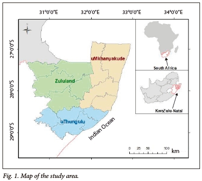
Three district municipalities in KZN, uMkhanyakude, uThungulu and Zululand, are malarious areas and were included in the study. The study areas are bordered by the countries of Swaziland and Mozambique to the north, and the Indian Ocean stretching from the east down to the southeast (Fig. 1). The province has a subtropical climate and most malaria cases occur during the rainy months from October to May, usually with a seasonal peak in January and March.8,9
Malaria data
We used confirmed monthly malaria cases including all age groups from January 2005 to December 2014, obtained from the KZN Malaria Control Programme. A malaria case is a person whose blood smear tested positive to Plasmodium after undergoing a rapid diagnostic test or slide microscopy at a health facility.10 Since 1956 it has been a legal requirement to notify malaria cases to the relevant health authorities in SA.11 Confirmed malaria cases at health facilities in the malarious provinces in SA are reported by telephone to the relevant district health office and subsequently reported to the provincial malaria control programme. At the provincial malaria control programme, the malaria control worker collects and inputs information relating to the malaria case into the malaria information system. The information includes patient demographics, the health facility where the case was reported, symptoms, malaria test results, diagnosis and treatment administered.8,12
No ethical approval for the study was required.
Statistical analysis
The analytical approach to this study is bounded by the Box-Jenkins SARIMA model. The SARIMA model combines non-seasonal and seasonal components, and can be specified as SARIMA (p,d,q) χ (P,D,Q)s, where p, d and q refer to the orders of the non-seasonal autoregressive (AR), non-seasonal differencing and non-seasonal moving average (MA) parts of the model. P, D and Q refer to the orders of the seasonal AR, seasonal differencing and seasonal MA parts of the model, and s is the length of the seasonal period. The AR process accounts for previously observed values up to a specified maximum lag, plus an error term. The process of differencing is referred to as the integration part that accounts for stabilisation of the data by removing seasonality or trend, while the MA process accounts for previous error terms, making forecasting easier. The algebraic form of the SARIMA model13 is given as:

The non-seasonal factors are given as:


The seasonal factors are given as:


where Xf= data series, at = random error (with mean zero and variance σ2, Β = backward shift operator, φ = coefficient non-seasonal autoregressive, θ = coefficient non-seasonal moving average, Φ = coefficient seasonal autoregressive, Θ = coefficient seasonal moving average, Δd = difference operator, with d order of differencing, and  = seasonal difference operator, with D seasonal order of differencing and s length of the seasonal period.
A SARIMA (p,d,q)(P,D,Q)12 model was constructed using monthly malaria case data from January 2005 to December 2013 and a forecast of malaria cases from January 2014 to December 2014, following the steps below.
Step 1: Transformation of time series data and model identification
The power transformation known as the Yeo-Johnson transformation was employed on the time series to stabilise the variance, while SARIMA non-seasonal and seasonal differencing were conducted to achieve stationarity of the time series by eliminating the trend and seasonality. From the non-seasonal and seasonal differenced data, the non-seasonal and seasonal components of the model were formulated by examining their autocorrelation function (ACF) an partial autocorrelation function (PACF). The ACF and PACF we e used to determine the degree of differencing and appropriate autoregressive and moving average terms.
Step 2: Parameter estimation
Parameters of the model in step 1 were estimated to verify that all the parameters in the plausible model were significant.
Step 3: Model validation
To test for the adequacy of the selected SARIMA model, we used the residuals of the fitted model to find the ACF plot of the residuals and the Box-Ljung test. The Q-Q plot and Shapiro-Wilk test were used to test for normality of the residuals. If all the diagnostic test results are within acceptable limits, the SARIMA model in step 2 is appropriate.
Step 4: Forecasting
The selected SARIMA model in step 3 was used to forecast malaria cases from January 2014 to December 2014. The reported malaria cases for 2014 were used to validate the forecast.
Results
Model identification
The time series data cover 120 months, from January 2005 to December 2015, and depict notable seasonality and a downward trend of malaria cases, as shown in Fig. 2 A.


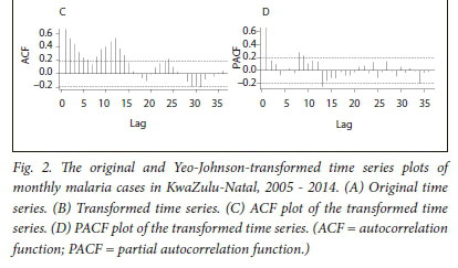
The Yeo-Johnson transformation method and differencing were employed to stabilise the variance and eliminate the seasonal trend, respectively.
The Yeo-Johnson transformation suppressed the fluctuations, which in turn enhanced the normality of the data (Fig. 2 B). The ACF plot of the transformed malaria case data in Fig. 2 C depicts seasonality, which dies down slightly, while the PACF plot of the malaria case data in Fig. 2 D tails off after lag 1, and decays in sine-wave fashion. In an initial attempt to remedy the non-stationarity of the time series (depicted in Fig. 2 B), and eliminate the trend and seasonality (indicated in the ACF plot in Fig. 2 C), non-seasonal differencing was employed.
In Fig. 3, A and B present the output of the monthly malaria cases after transformation and non-seasonal differencing. The ACF plot in Fig. 3 A indicates that seasonality is still evident (lags 7, 19 and 31).

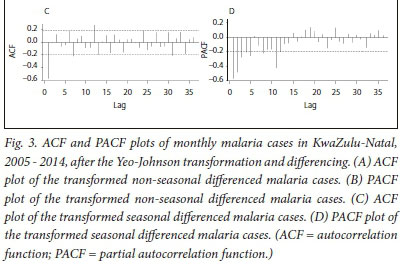
We therefore employed seasonal differencing to eliminate the effect of seasonality in our model and to seek for a better model fit.
The non-seasonal component of our model was identified by examining the ACF and PACF plots (Fig. 3 A and B) of the transformed non-seasonal differenced malaria cases. The ACF values in Fig. 3 A decline steadily after 1 lag and the PACF (Fig. 3 B) decays exponentially in a sine-wave fashion. This suggests a moving average of order 1, resulting in an autoregressive moving average (0,1,1)12 model (i.e. p = 0, d = 1 and q = 1).
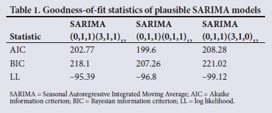
In Fig. 3, C and D show the ACF and PACF plots of monthly malaria cases after transformation and seasonal differencing. In Fig. 3 C, the ACF cuts off after 1 lag, which suggests a seasonal moving average MA (1) model, while the PACF plot (Fig. 3 D) declines after 3 lags, which suggests a seasonal autoregressive AR (3) model. Therefore, based on the non-seasonal differencing and seasonal differencing, seasonality was eliminated from the time series data and a stationary mean (i.e. D = 0) was achieved. This resulted in the identification of three plausible SARIMA models, SARIMA (0,1,1) (3,1,1)12, SARIMA (0,1,1)(0,1,1)12, and SARIMA (0,1,1)(3,1,0)12.
Model testing and parameter estimation
The goodness-of-fit statistics employed were the Akaike information criterion (AIC), the Bayesian information criterion (BIC), log-likelihood and the standard error. The model with the lowest BIC value and with a p-value <0.05 was selected as the best model fit. The BIC values are based on the likelihood function and the AIC.6 The SARIMA (0,1,1)(0,1,1)12 model has the smallest BIC (Table 1) and all the estimates provided in Table 2 are significant. Therefore, based on the goodness-of-fit statistics (Table 1) and parameter estimation (Table 2), we identified the SARIMA (0,1,1)(0,1,1)12 model as the most suitable model for forecasting.
Model validation
This was done by verifying: (i) the ACF of the residuals to check for autocorrelation; and (ii) the normal probability plot of the residuals.
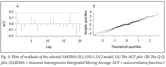
The ACF plot of residuals (Fig. 4, A) suggests that the residuals have a constant variance, and the autocorrelations were modelled out leaving only one significant value as indicated by the spike in lag 19. Also, the Box-Ljung test results (χ2 = 60.499, df = 48, p-value = 0.1064) revealed that the p-value exceeded 5%, implying that the model is adequate (i.e. there is no autocorrelation). The Shapiro-Wilk test results for normality have a test statistic of W=0.98811 and p-value of 0.4595, and the Q-Q plot (Fig. 4, B) depicts some outliers on the tails, suggesting that the normality of the residuals is not rejected. We therefore proceeded to use the SARIMA (0,1,1)(0,1,1)12 model for forecasting, since it provides a reasonable fit to the highly seasonal and non-seasonal time series data.
Forecasting
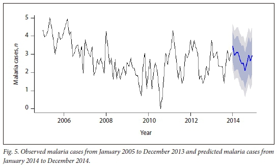
The selected SARIMA (0,1,1)(0,1,1)12 model was used to forecast monthly malaria cases from January 2014 to December 2014 (Fig. 5).
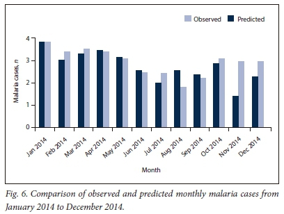
The plot of the observed monthly malaria cases and predicted cases for 2014 (Fig. 6) shows that the values for monthly predicted cases tend to follow the reported values quite closely except in August, November and December, where pronounced differences were observed.
Discussion
Time series predictions are generated by models based on changes over time in previously observed values or historical datasets.14 The SARIMA forecast model can serve as a useful tool for public health workers and epidemiologists. It can be applied as a malaria early-warning system and, can provide vital information to enable the relevant authority to act proactively.14,15This study shows how the SARIMA model (which is particularly relevant for a disease that exhibits seasonality) was employed in modelling and predicting malaria cases in a relatively low malaria transmission region, where targeted interventions are vital to strengthen KZN malaria control and elimination efforts. The model can provide information to support policy makers and public health efforts so that intervention resources can be provided and chanelled in a sustainable and effective way. It can also serve as a tool for providing relevant information to locals and visitors prior to high malaria transmission months. This in turn will be pivotal in transforming SA's current malaria programme to elimination by 2020.
The epidemiological potential and functionality (epidemiological studies, disease surveillance and forecasting) of the SARIMA time series have been explored by various authors in different capacities.16-20 These authors ensured that the time series processes attained stationarity in the homogenous sense (stationary in its level) and variance, which are indispensable conditions of a SARIMA model. This was done by carrying out the first differencing and the seasonal differencing, which results in a stationary time series by removing trends and seasonal effects. However, in instances where the variance of a time series trends downwards (or increases) as the level of the series decreases (or increases), the time series must be transformed before the analysis or differencing.14 This will lead to a time series stationary in the homogenous sense and variance, and in turn improves and leads to the formulation of a better model fit.14 Some studies employed log-transformation to achieve a stationary variance,21-23 and this is the most commonly used transformation approach. Other studies employed Box-Cox power transformation,24,25 which is valid for datasets containing positive variables. In this study, we employed a seldom-used power transformation known as the Yeo-Johnson transformation because our time series systematically trended downwards and had zero values and values close to zero.26
Although malaria transmission in KZN is limited as a result of effective malaria control measures,9,27-29 the SA National Department of Health still regards malaria as a significant disease owing to its propensity to cause an epidemic.8,10In SA, specific population groups are at higher risk of contracting malaria. They are infants and children aged <5 years living in localities of stable malaria transmission, the elderly (>65 years old), people living with HIV/AIDS, non-immune pregnant women, semi-immune pregnant women living in high malaria transmission localities, semi-immune HIV-infected pregnant women living in localities of stable transmission, non-immune travellers and migrants.10Nevertheless, the entire population is vulnerable to malaria epidemics owing to little or no immunity.10 To avert an epidemic, SA has in place an outbreak threshold of confirmed cases at districts and provinces endemic to malaria, and health facilities located in these areas. When the threshold is reached or exceeded, reactive measures are taken by the relevant malaria divisions.8-The malaria control and elimination efforts needed will therefore require scaling up and revising of the epidemic preparedness and response strategy.
In addition to our SARIMA model, further studies should be conducted utilising either epidemiological or entomological data or a combination of both, with environmental and socioeconomic malaria triggers at a fine scale to delineate the intervention resources needed. Furthermore, conducting epidemiological research, and studies in a particular setting employing different parameters, mechanisms or possible confounders, can inform us on the deficiencies in our knowledge of malaria disease in that study area. This could result in the identification of unanswered questions and loopholes crucial to model reliability, which can be bridged by either incorporating more variables or eliminating certain variables. Nevertheless, without practical applications of developed models, we will not be informed about the reliability of the models and how they can be improved. It is also important to bring relevant stakeholders (researchers, statistical analysts, the South African Weather Service, doctors, public health workers, epidemiologists, entomologists and policy makers) together to reshape the malaria elimination strategy so that reliable and operational malaria case prediction models can be generated. Such multidisciplinary collaboration will also enable reliable malaria predictors and accurate hotspots of malaria transmission to be identified.30 In addition, a reliable and direct means of accessing and sharing information among the relevant stakeholders is of the utmost necessity.
Study limitations
The weakness of this study is that it attempted to develop a single model for the entire malarious area of KZN. Separate models for each of the district municipalities could provide an in-depth assessment of the malaria trends across the district, which in turn might help identify possible differences in the implementation of prevention measures, patients' seeking behaviours and migration of people. The structuring of our data and the mode of the forecasting (using monthly data and forecasting) may be responsible for the overestimated and underestimated monthly forecast observed. Conducting daily data analysis could result in improved model fit and daily forecasts, which could then be aggregated into weekly and monthly forecasts. The univariate analysis approach employed in this study could be another reason for the overestimated and underestimated forecasts. The incorporation of independent-variable time series into the SARIMA model (multivariate SARIMA model) over a longer time frame could improve the model fit and the forecast if the exogenous factors responsible for trend, seasonality and outliers are incorporated into the model.
Conclusions
The SARIMA forecast model is a valuable tool that has the potential for malaria early warning and early detection in KZN, SA. It can provide reliable information to the relevant authority to act pro-actively, because the values of the malaria forecast from the best fit SARIMA (0,1,1)(0,1,1)12 model fitted closely with the values of the reported malaria cases. Nevertheless, the practical application of the generated model is encouraged. Furthermore, studies that employ daily data and incorporate possible malaria transmission risk factors and confounders in multivariate time-series models are recommended.
Acknowledgements. We thank the College of Agriculture, Engineering and Science of the University of KwaZulu-Natal for the doctoral research bursary awarded to OE. We also thank the Malaria Control Programme, Jozini, KwaZulu-Natal for providing the malaria data. Author contributions. OE and MG conceived and designed the study, OE and MG contributed to data acquisition, OE and LM did statistical analysis and interpretation, OE drafted the initial manuscript, and MG and LM critically revised the manuscript. All authors read and approved the final manuscript. Funding. None. Conflicts of interest. None.
References
1. World Health Organization. Malaria Country Profile 2016. Geneva: WHO, 2016. http://www.who.int/malaria/publications/country-profiles/en/ (accessed 11 September 2017). [ Links ]
2. Elimination 8. Annual Report 2016. Windhoek: E8, 2016. https://malariaelimination8.org/wp-content/uploads/2017/05/e8-annual-report-2016.pdf (accessed 11 September 2017). [ Links ]
3. Raman J, Morris N, Frean J, et al. Reviewing South Africa's malaria elimination strategy (2012 - 2018): Progress, challenges and priorities. Malaria J 2016;15(1):438. https://doi.org/10.1186/s12936-016-1497-x [ Links ]
4. Cunha GB, Luitgards-Moura JF, Naves EL, Andrade AO, Pereira AA, Milagre ST. Use of an artificial neural network to predict the incidence of malaria in the city of Canta, state of Roraima. Rev Soc Bras Med Trop 2010;43(5):567-570. https://doi.org/10.1590/S0037-86822010000500019 [ Links ]
5. Zinszer K, Verma AD, Charland K, et al. A scoping review of malaria forecasting: Past work and future directions. BMJ Open 2012;2(6):e001992. https://doi.org/10.1136/bmjopen-2012-001992 [ Links ]
6. Chatfield C. The Analysis of Time Series: An Introduction. 6th ed. Florida: CRC Press, 2003. [ Links ]
7. Shumway R, Stoffer D. Time Series Analysis Using the R Statistical Package. Free Dog Publishing, 2017. http://www.stat.pitt.edu/stoffer/tsa4/tsaEZ.pdf (accessed 10 November 2017). [ Links ]
8. National Department of Health, South Africa. Republic of South Africa Malaria Elimination Strategy 2011 - 2018. Pretoria: NDoH, 2012. [ Links ]
9. Moonasar D, Nuthulaganti T, Kruger PS, et al. Malaria control in South Africa 2000 - 2010: Beyond MDG6. Malaria J 2012;11(1):294. https://doi.org/10.1186/1475-2875-11-294 [ Links ]
10. National Department of Health, South Africa. Guidelines for the Treatment of Malaria in South Africa - 2016. Pretoria: NDoH, 2016. [ Links ]
11. National Department of Health, South Africa. Notification of Diseases. Pretoria: NDoH, 1956. [ Links ]
12. Khosa E, Kuonza LR, Kruger P, Maimela E. Towards the elimination of malaria in South Africa: A review of surveillance data in Mutale Municipality, Limpopo Province, 2005 to 2010. Malaria J 2013;12(1):7. https://doi.org/10.1186/1475-2875-12-7 [ Links ]
13. Brockwell, PJ, Davis RA. Time Series: Theory and Methods. New York: Springer Science & Business Media, 1991. [ Links ]
14. McCleary R, Hay RA, Meidinger EE, McDowall D. Applied Time Series Analysis for the Social Sciences. Beverly Hills, Calif.: Sage Publications, 1980. [ Links ]
15. Midekisa A, Senay G, Henebry GM, Semuniguse P, Wimberly MC. Remote sensing-based time series models for malaria early warning in the highlands of Ethiopia. Malaria J 2012;11(1):165. https://doi.org/10.1186/1475-2875-11-165 [ Links ]
16. Dan ED, Jude O, Idochi O. Modelling and forecasting malaria mortality rate using Sarima models (a case study of Aboh Mbaise general hospital, Imo State Nigeria). Sci J Appl Math Stat 2014;2(1):31-41. https://doi.org/10.11648/j.sjams.20140201.15 [ Links ]
17. Kumar V, Mangal A, Panesar S, et al. Forecasting malaria cases using climatic factors in Delhi, India: A time series analysis. Malaria Res Treat 2014; Article ID 482851. https://doi.org/10.1155/2014/482851 [ Links ]
18. Permanasari AE, Hidayah I, Bustoni IA. SARIMA (Seasonal ARIMA) implementation on time series to forecast the number of malaria incidence. International Conference on Information Technology and Electrical Engineering (ICITEE), 7 - 8 October 2013, Yogyakarta, Indonesia. Yogyakarta: IEEE, 2013:203-207. https://doi.org/10.1109/iciteed.2013.6676239 [ Links ]
19. Briët OJ, Vounatsou P, Gunawardena DM, Galappaththy GN, Amerasinghe PH. Models for short term malaria prediction in Sri Lanka. Malaria J 2008;7(1):76. https://doi.org/10.1186/1475-2875-7-76 [ Links ]
20. Wangdi K, Singhasivanon P, Silawan T, Lawpoolsri S, White NJ, Kaewkungwal J. Development of temporal modelling for forecasting and prediction of malaria infections using time-series and ARIMAX analyses: A case study in endemic districts of Bhutan. Malaria J 2010;9(1):251. https://doi.org/10.1186/1475-2875-9-251 [ Links ]
21. Zinszer K, Kigozi R, Charland K, et al. Forecasting malaria in a highly endemic country using environmental and clinical predictors. Malaria J 2015;14(1):245. https://doi.org/10.1186/s12936-015-0758-4 [ Links ]
22. Homan T, Maire N, Hiscox A, et al. Spatially variable risk factors for malaria in a geographically heterogeneous landscape, western Kenya: An explorative study. Malaria J 2016;15(1):1. https://doi.org/10.1186/s12936-015-1044-1 [ Links ]
23. Krefis AC, Schwarz NG, Krüger A, et al. Modeling the relationship between precipitation and malaria incidence in children from a holoendemic area in Ghana. Am J Trop Med Hyg 2011;84(2):285-291. https://doi.org/10.4269/ajtmh.2011.10-0381 [ Links ]
24. Trebbia G, Lacombe M, Fermanian C, et al. Cough determinants in patients with neuromuscular disease. Resp Physiol Neurobiol 2005;146(2):291-300. https://doi.org/10.1016/j.resp.2005.01.001 [ Links ]
25. Ren Z, Wang D, Hwang J, et al. Spatial-temporal variation and primary ecological drivers of Anopheles sinensis human biting rates in malaria epidemic-prone regions of China. PLoS One 2015;10(1):e0116932. https://doi.org/10.1371/journal.pone.0116932 [ Links ]
26. Yeo IK, Johnson RA. A new family of power transformations to improve normality or symmetry. Biometrika 2000;87(4):954-959. https://doi.org/10.1093/biomet/87.4.954 [ Links ]
27. Ebhuoma O, Gebreslasie M, Magubane L. Modeling malaria control intervention effect in KwaZulu-Natal, South Africa using intervention time series analysis. J Infect Public Health 2017;10(3):334-338. https://doi.org/10.1016/j.jiph.2017.02.011 [ Links ]
28. Maharaj R, Mthembu DJ, Sharp BL. Impact of DDT re-introduction on malaria transmission in KwaZulu-Natal. S Afr Med J 2005;95(11):871-874. [ Links ]
29. Maharaj R, Raman J, Morris N, et al. Epidemiology of malaria in South Africa: From control to elimination. S Afr Med J 2013;103(10):779-783. https://doi.org/10.7196/SAMJ.7441 [ Links ]
30. Ebhuoma O, Gebreslasie M. Remote sensing-driven climatic/environmental variables for modelling malaria transmission in Sub-Saharan Africa. Int J Environ Res Public Health 2016;13(6):584. https://doi.org/10.3390/ijerph13060584 [ Links ]
 Correspondence:
O Ebhuoma
osadolorebhuoma@gmail.com
Accepted 11 December 2017

