


Services on Demand
Article
 English (pdf)
 Article in xml format
 Article references
Indicators

Related links
-
 Cited by Google
 -
 Similars in Google
Share

 Permalink
Koedoe
On-line version ISSN 2071-0771
Print version ISSN 0075-6458
Koedoe vol.60 n.1 Pretoria 2018
http://dx.doi.org/10.4102/koedoe.v60i1.1497
ORIGINAL RESEARCH
The 2013-2014 vegetation structure map of Hwange National Park, Zimbabwe, produced using free satellite images and software
Eduardo M. ArrautI, II, III, IV; Andrew J. LoveridgeI, V; Simon Chamaillé-JammesVI, VII, VIII; Hugo Valls-FoxVI, VII, IX, X; David W. MacdonaldI
IWildlife Conservation Research Unit, Department of Zoology, Oxford University, United Kingdom
IIDepartment of Water Resources and Environment, Aeronautics Institute of Technology, Brazil
IIIDivision of Remote Sensing, National Institute for Space Research, Brazil
IVDepartment of Plant Biology, State University of Campinas, Brazil
VLady Margaret Hall, Oxford University, United Kingdom
VICEFE, CNRS, Univ. Montpellier, Univ. Paul Valéry Montpellier 3, EPHE, IRD, Montpellier, France
VIILTSER-France, Zone Atelier 'Hwange', Hwange National Park, Zimbabwe
VIIIDepartment of Zoology & Entomology, University of Pretoria, South Africa
IXCIRAD, UMR SELMET, Montpellier, France
XSELMET, Univ Montpellier, CIRAD, INRA, Montpellier SupAgro, Montpellier, France
ABSTRACT
Vegetation mapping of protected areas is a cornerstone of conservation worldwide. Established in 1928 and covering over 1.4 million hectares, Hwange National Park (HNP) is the largest natural reserve in Zimbabwe. In 1993, the sole comprehensive map of its vegetation to date was produced and since then it has been used in numerous research and conservation endeavours. Over the last two decades, however, the park's vegetation changed, safari areas and forest reserves were created at its edge and high-positional accuracy data on a suite of species were collected. To tend to contemporary mapping needs, in this article, we present the 2013-2014 vegetation structure map of HNP and its surroundings. It was produced by supervised classification of Landsat-8 Operational Land Imager (OLI) images, indices derived from these and the Landsat Tree Cover Continuous Field product. Its accuracy was assessed statistically using samples collected from high-resolution satellite imagery and basic ancillary field data. Of its total pixels, 83.2% were correctly classified. Mean omission and commission error were, respectively, 0.82 (0.74-0.90) and 0.82 (0.72-0.89), and this similarity held on a per class basis, indicating reliable area estimates. It was produced using only freely available imagery and software.
Conservation implications: In addition to providing researchers and conservationists working within and around HNP with an updated vegetation map, aiming at an even broader audience, we provide a step-by-step approach for using modern freely available imagery and software for cost-effectively mapping HNP in future or other protected savannas across Africa.
Introduction
Vegetation mapping of protected areas and their surroundings has been a cornerstone of conservation planning and management worldwide (Freemantle et al. 2013; Pettorelli, Safi & Turner 2014; Rose et al. 2015). In Africa, for example, it has allowed for inferring the health of the threatened Miombo woodlands of Mozambique (Sedano, Gong & Ferrão 2005), assessing the large-scale impacts of herbivores upon the structural diversity of Kruger National Park's vegetation (Asner et al. 2009), predicting the risk of African lion (Panthera leo) attacks on humans in Tanzania (Kushnir et al. 2014) and planning of the Great Limpopo Transfrontier Conservation Area (Martini et al. 2016). Such mapping has also been at the heart of conservation initiatives in South America (Oliveira et al. 2017), Asia (Davies, Murphy & Bruce 2016), Europe (Palomo et al. 2013) and North America (Wiens et al. 2009).
Hwange National Park (HNP), covering an area of over 1.4 million hectares, is the largest protected area in Zimbabwe and part of the Kavango-Zambezi Transfrontier Conservation Area (The Government of the Republic of Angola et al. 2011). It is home to rich biodiversity and adjacent to important land concessions (Loveridge, Reynolds & Milner-Gulland 2007a, Loveridge et al. 2007b). To our knowledge, since HNP's establishment in 1928, three maps of its vegetation has been produced. The first one, of the Robins area, was based on aerial photography and the vegetation was manually classified (Robinson, Hill & Rushworth 1973). Twenty years later, similar data were used to produce the park's first comprehensive map of major vegetation types and structures (Rogers 1993). For the following two decades, this was the reference map in studies concerning lions (Davidson et al. 2012; Loveridge et al. 2009; Valeix et al. 2009), jackals (Canis mesomelas and Canis adustus) (Loveridge & Macdonald 2002), elephants (Loxodonta africana) and other herbivores (Chamaillé-Jammes et al. 2008; Periquet et al. 2012; Valeix et al. 2011). The more recent map, which covers a third of the park, was made using Landsat Thematic Mapper images acquired in 2002-2003 and used to study the responses of zebras (Equus quagga) to lion encounters (Courbin et al. 2016).
The map introduced in this study represents the status of the vegetation structure in 2013-2014, thus representing a 20-year update in the park's mapping, and encompasses HNP plus a 50 km buffer around it, to which safari areas, forest reserves, communal lands and research and conservation endeavours have expanded in the last decade. In addition, the map herein was subject to a statistical accuracy assessment, making it particularly suitable for analyses involving the modern geo data sets that come with positional precision estimates, such as Global Positioning System (GPS) telemetry, and which have been collected on a suite of species living in HNP over the last two decades. In addition to budgetary constraints, its production required overcoming challenges related to (1) difficulty of visiting remote areas on the ground, (2) marked differences in ground colour because of soil and fire and (3) asynchronicity in phenology. As explained earlier, we overcame these using free images, products and software. We believe that our procedure could be used for retrospective analyses of vegetation change in HNP and the production of future maps of the area, as well as for mapping similar classes of savanna vegetation structure within and around other protected areas. We hope the detailed information concerning the making of a vegetation structure map 'from scratch' provided here may represent a case study for practitioners with similar needs elsewhere.
Research method and design
Setting: Study area
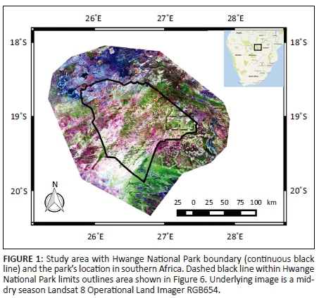
The 46 207 km2 study area includes HNP (14 651 km2) and adjacent safari areas, forest reserves and communal lands in Zimbabwe and Botswana within a 50 km buffer around HNP (Figure 1). The vegetation is typical of a highly heterogeneous dystrophic wooded savanna (Figure 2). Overall, woody cover increases with distance from water pans (Chamaillé-Jammes, Fritz & Madzikanda 2009). Sandy soils, locally known as Kalahari sands, that cover about two-thirds of HNP are generally dominated by Baikiaea plurijuga woodlands or a mixed bushland community dominated by Combretum spp., Terminalia sericea and a few Acacia spp. groves, with open grasslands along drainage lines. To the north, basaltic and clayey soils are dominated by woody species, such as Colophospermum mopane bushland or woodlands (Rogers 1993). Outside the HNP, additional vegetation types include farmlands and extensive wetlands and seasonal riverbeds to the south-east. Altitude throughout the study area varies from c. 835 m to c. 1200 m above sea level. Annual rainfall is highly variable (coefficient of variation = 25%) around a mean of 600 mm. Rains predominate between November and February (Chamaillé-Jammes, Fritz & Murindagomo 2006), with numerous water pans being formed during the rainy season and most drying out completely in the dry season. To sustain animals during the dry season, within HNP, underground water is pumped to some artificial waterholes (Chamaillé-Jammes, Fritz & Murindagomo 2007).
Materials
Field data
The field protocol consisted of visiting sites, making schematic diagrams and taking geotagged photos. Field sites were representative of vegetation structure classes and underlying ground signals (see Figure 2). Their locations were chosen based on expert knowledge and accessibility by car or on foot. Geotagged photos were taken of the 208 field sites visited, while 76 diagrams were made. The purpose of making diagrams was to oblige the researcher to carefully observe and record on paper the surroundings of a field site. This information would later aid interpretation of the photos.
Satellite image data and products
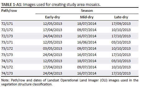
Only free images and products were used in the study. These included 30 m × 30 m resolution bands 2-6 of 27 Landsat 8 (L8) Operational Land Imager (OLI) images (see Appendix 1), downloaded from the EarthExplorer website (https://earthexplorer.usgs.gov/), and the 2005 Vegetation Coninuous Fields (VCF) Tree Cover product (Sexton et al. 2013), available at NASA's Global Land Cover Facility (http://glcf.umd.edu/data/landsatTreecover/).
Thematic classes used in classification
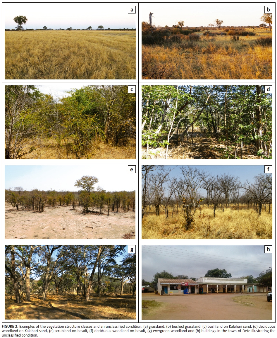
The vegetation structure classes were (1) grassland, (2) bushed grassland, (3) bushland on Kalahari sand, (4) deciduous woodland on Kalahari sand, (5) scrubland on basaltic soil, (6) deciduous woodland on basaltic soil and (7) evergreen woodland (these numbers are used to refer to these classes elsewhere in the article; classes with no associated soil class name occurred on both soil types). However, these were not the actual classes on which the classification was based because during fieldwork we identified three confounding factors: (1) difference in the reflective properties of the two major soil types, (2) fire and (3) asynchronicity in phenology. The effect of the difference in soil type was more prominent in the dry season images, when the weaker signal of the dry vegetation led to an increase in the relative contribution to pixel reflectance of the underlying soil signal. As the classification required multitemporal images and different vegetation structure classes had the same underlying soil type, this played towards reducing their spectral separability. Burning reduced dramatically the reflectance of the target, and because it happened to different vegetation classes, it also contributed to reducing their separability. Finally, asynchronicity in phenology implied that the same vegetation structure class appeared vigorous and dry in the same image, resulting in an increase in intra-class variance, and hence, a reduction in inter-class separability. To solve these issues, the classification was carried out considering a subdivision of the desired vegetation classes into 'spectral classes'. These were composed of the above vegetation structure classes plus the classes 'bare grassy areas near waterholes', 'grassland, burnt', 'deciduous woodland on Kalahari soil, burnt' and 'scrubland on basaltic soil, burnt'. As will be explained later, these spectral classes were grouped into the desired vegetation structure classes during post-processing.
Procedure
A summary of the steps for producing the final map is presented in Figure 3.
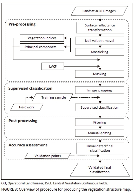
Image visual and digital processing were carried out using GRASS 7.0 (GRASS 2012) and QGIS Desktop 2.8 with the GRASS 6.4 plugin (Development Team QGIS 2015). GRASS 7.0 was used mainly during pre-processing, and classification and initial post-processing steps (filtering), while QGIS 2.8 with the GRASS 6.4 plugin was used mainly during late post-processing (manual editing and merging edited layer with original classification) and accuracy assessment (Figure 3). Geotagged photos were imported using the Photo2Shape plugin in QGIS (Bruy 2013), which creates a georeferenced point vector layer of each photo. The OpenLayers QGIS plugin (Sourcepole 2014) was used to visualise high-resolution Quickbird images from Google Earth during the response sample definition (see 'Accuracy assessment' section). A general introduction to the newest GRASS manual, which contains the explanations and algorithms regarding image classification, may be found on the Internet - at time of this publication, it was GRASS 7.4 (GRASS 2017).
Pre-processing
The first step was to convert each band of each scene to surface reflectance using the i.landsat.toar function with DOS4 option enabled and parameter values set from the metadata file downloaded with each scene. This particular algorithm reports at-surface reflectance by, firstly, performing a radiometric calibration (using gain and bias parameters) and then correcting for acquisition geometry (using estimates for the distance from the sun, solar elevation angle and mean solar exoatmospheric irradiance) and, secondly, removing atmospheric path radiance (scattering) with the dark object method (Chavez 1988; Vincent 1972). The i.landsat.toar sets pixels in the image's bounding square to zero, which is a problem for the mosaicking algorithm used later (it considers them meaningful values). To avoid this, the r.null function was applied to them. Then, the r.patch function was used to produce three mosaics with nine scenes each, for early-dry, mid-dry and late-dry seasons. As at the time, the GRASS algorithms could not handle 16-bit images, all mosaics were converted from 16 to 8 bit. True colour RGB432 and false colour RGB645 composites were then produced.
We then used the GRASS function i.vi to produce the Enhanced Vegetation Index 2 (EVI-2) (Jiang et al. 2008) and the Soil Adjusted Vegetation Index (SAVI) (Huete 1988), and i.pca to produce the first, second and third principal components of the late-dry season OLI bands. The EVI-2 and SAVI were used, respectively, to help differentiate classes during the early- and mid-dry seasons, when they are useful for differentiating green vegetation with different metabolism and canopy structure, and during the late-dry season, when the soil signal from underneath the dry vegetation is more noticeable. The principal components were made to further aid the differentiation of classes during the dry season.
To define the study region, a mask corresponding to HNP plus a 50 km boundary strip was applied using the r.mask function in GRASS.
Supervised classification
Image grouping: In GRASS geographic information system (GIS), all training sample statistics and classifications are performed on image groups and subgroups, which are defined using the function i.group. An image group is a named collection of raster layers and a subgroup is a specific combination of the layers present in the group. By varying the subgroup used in each of a series of preliminary classifications, the user can test which combinations of layers within a group yield the best results.
Training sample: Training sample was created using field information, high-resolution Quickbird images available freely in Google Earth, the LVCF and the Landsat-8 OLI bands from wet, early-, mid- and late-dry seasons. To define the samples, a vector layer was created in GRASS 6.4 with a column 'cover' representing a code for each land-cover class. The function v.edit was used to create the polygons delimiting training sample acquisition. This vector layer was then converted to raster using v.to.rast, with the source of raster values (the land-cover class) coming from the column 'cover'. This new raster layer was used as the reference map. It delimited areas in space from which sample statistics were derived from the image subgroups. The final training sample was defined after an iterative process in which classifications involving training samples with progressively greater per-class variance were visually contrasted, that is, one begins by classifying using samples obtained from pixels representing homogeneous areas of each vegetation type and at every step adds variance to each sample by including pixels located at class transition zones.
Supervised classification: Supervised classification was carried out using the Bayesian multiscale random field sequential maximum a posteriori (SMAP) classifier available in GRASS 7.0 (Bouman & Shapiro 1994; McCauley & Engel 1995). When classifying a pixel, this classifier considers information from its contiguous neighbours and checks that the class assigned to it appears consistent by sequentially comparing which classes predominate in a set of larger neighbourhoods around this pixel. This effectively implies that it classifies a pixel based on information about the land-cover patch within which it is situated. Sequential maximum a posteriori classifiers have been shown to perform better than classifiers based on maximum likelihood (ML) or other Bayesian-based approaches (Bouman & Shapiro 1994; McCauley & Engel 1995); we confirmed this by carrying out preliminary classifications using the ML algorithm also available in GRASS and using our field data and knowledge to visually compare its results with those produced by SMAP. To carry out the classification, firstly, class statistics were generated using the i.smap function and using the raster reference map and subgroups mentioned above. This created the signature file, which contained the reference statistics for each of the classes to be used in the classification. Secondly, contextual image classification using SMAP estimation was performed by the function i.smap using the aforementioned groups and signature file.
Post-processing
The function r.neighbors was used to apply 3 × 3, 5 × 5, 7 × 7, 9 × 9 and 11 × 11 median neighbourhood filters to the final classification. Median filters reduce classification noise without altering class values (in contrast to, for example, a mean filter, which alters class values). To the best of our judgement, the 5 × 5 filter yielded the better results and therefore the classification to which we applied it was chosen as the final map. Then, manual vector editing was performed to assign the correct class to some areas that had been so recently and intensely burnt that the classifier confounded them with water (which has extremely low reflectance in the L8 bands we were using). Virtually all of the edited area fell outside HNP and it amounted to approximately 3% of the total mapped area and about 20% of the total recently burnt area (as estimated using QGIS to manually delimit burnt areas in the late-dry season image). For this purpose, a vector layer was created in QGIS and polygons with attribute values defining the new classes were created. The rasterise function in QGIS was then used to merge these polygons with the unedited raster classification, thus producing the map to be subject to accuracy assessment.
Accuracy assessment
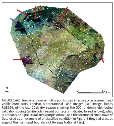
Accuracy assessment was carried out following nomenclature and recommendations by Olofsson et al. (2014) and Stehman and Czaplewski (1998). The sampling unit was the vector point, and the sampling design, which is the method by which the sampling units are chosen from the statistical population (the map), consisted of placing 500 points on the map using a simple random sampling scheme (distribution of the points shown in Appendix 2). The distribution of points across classes was then compared to the distribution of class areas and their similarity indicated that the scheme had not favoured any class. This illustrates a key property of a simple random sampling scheme, which is not to attribute importance to any class a priori. As a consequence, the interpretation of overall and class probabilities becomes straightforward: (1) global accuracy can be translated into the probability that a point on the map was correctly classified, (2) producer's accuracy (omission error) to the probability that a patch of a certain vegetation structure type was correctly classified and (3) user's accuracy (commission error) to the probability that a patch of a map class represents the correct cover type.
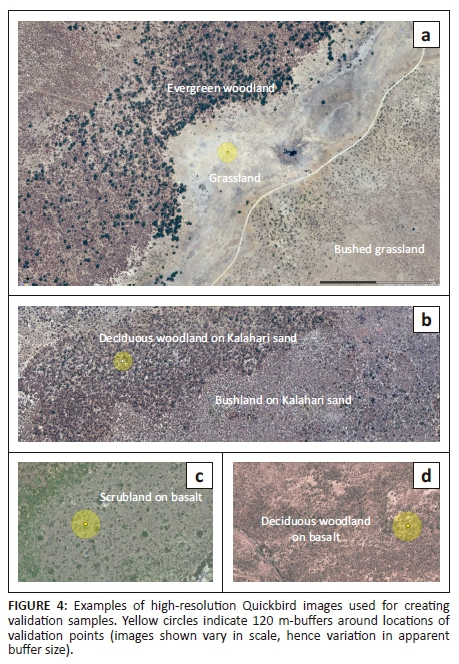
The response design, which is the protocol by which the reference class is associated with each sampling unit, consisted of attributing, to the point, the class predominating within a 60 m radius centred on it (Figure 4). This buffer size was chosen to minimise co-registration errors. The assessment of which class predominated within a buffer was made using high-resolution Quickbird images (Figure 4), aided by all other satellite and field data and information available (including a data set of images from camera-traps deployed throughout most of HNP). The computation of statistics was carried out using the r.kappa algorithm, which produced the confusion matrix and calculated classes' accuracy statistics and overall percentage of correctly classified pixels. Global, producer and user accuracies were then estimated from the confusion matrix. As several scientific studies are restricted to within HNP limits, in addition to assessing the accuracy of the entire mapped area, we also estimated each of the accuracy parameters for the area restricted to within the park's limits (n = 198 points).
Results
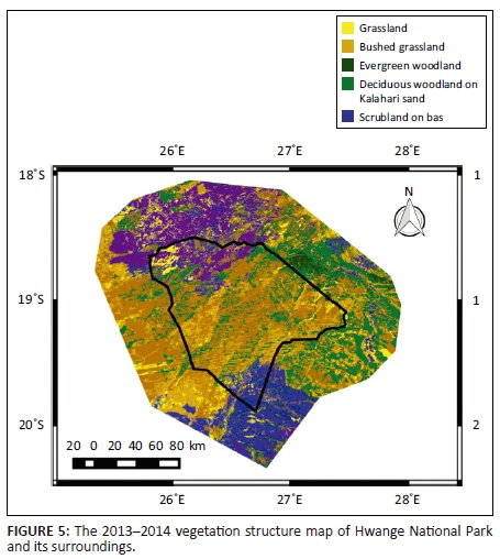
The 2013-2014 vegetation structure map of HNP and its surroundings is shown in Figure 5.
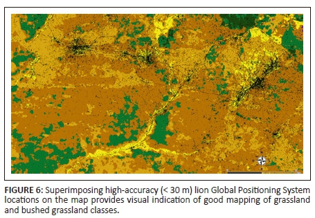
As an example of the map's ability to capture areas that are vital for one of HNP's most emblematic species, Figure 6 shows how lion GPS locations fell within the grassland and bushed grassland areas that these animals regularly use for resting, foraging and commuting between waterholes.
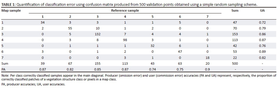
Of the 500 samples used in validation, 83.2% were classified correctly (Table 1), and when only the 198 validation points that fell within HNP were considered, this percentage increased to 89.9%. As this map was validated using a simple random sampling scheme, the measures of global accuracy can be interpreted as the chance that a randomly chosen pixel (0.09 ha) was correctly classified.
Producer accuracies (PAs) varied between 0.90 and 0.74 (mean = 0.83; standard deviation [SD] = 0.06) and user accuracies (UAs) between 0.89 and 0.72 (mean = 0.822; SD = 0.06), and the per-class difference (in modulus) between them varied between 0.15 (grassland) and 0.00 (deciduous woodland on Kalahari), suggesting class area estimates were reliable (the smaller the difference, the more reliable the area estimate). The two classes that conformed less to this pattern were 1 (grassland), with PA versus UA = 0.15, and 6 (deciduous woodland on basalt), with PA versus UA = 0.14. In class 1, higher PA (0.87) than UA (0.72) indicated that most grassland patches were correctly identified, but overall class area was slightly overestimated by attribution of this class to patches covered by other types, namely, bushed grassland, bushland and deciduous woodland on basalt (Table 1). These classes are characterised by a continuous underlying grass cover in places where shrubs or trees are sparse. In such areas, the signal from the LVCF gets weaker and that from the grasses becomes stronger, resulting in a preponderance of the latter and hence confusion with the grassland class. Conversely, in class 6, the lower PA (0.75) and higher UA (0.89) suggested that this vegetation structure type was rarely wrongly mapped, but that patches where it occurs were sometimes assigned to other classes, implying that its area was marginally underestimated. Final estimates for the area occupied by each vegetation structure class are presented in Table 2.

Discussion
The map introduced in this article depicts the state of the vegetation in HNP and surrounding reserves and land concessions in 2013-2014 (Figure 5), 20 years more recently than the previous map of the entire park (Rogers 1993). The vegetation classes distinguished in it are rather broad classes defined on the basis of vegetation structure. In particular, the classes reflect variability in openness and vegetation height, which we consider to have important and numerous functional consequences. For instance, in our own work on large mammal ecology, we have previously shown that dense and bushy areas where visibility is low, rather than dense woodlands where visibility is greater, are selected for by lions, which are ambush predators (Davidson et al. 2012). Thus, we think that the classes identified should be useful to map and understand functional processes at the landscape scale. Also, the map produced here offers baseline data to monitor, at a large scale, changes in these key variables (openness and height). In HNP, this is particularly important in the face of the persistence of a large elephant population that may affect vegetation structure in the long run (Valeix et al. 2011).
As this map was validated via a simple random sampling scheme, its classes can be combined to create other maps with global and per-class accuracy statistics easily calculable from the original confusion matrix. Thus, if, for example, the grassland and bushed grassland classes should be grouped into the 'open areas' class, which has been shown to be strongly selected for by zebras (Courbin et al. 2016), this new class would have PA = 0.89 and UA = 0.80 (n = 117). For a recent review of the applicabilities and limitations of other accuracy assessment schemes, most of which can be quite easily implemented using freely available GIS (Development Team QGIS 2015; GRASS 2012; see Methods section), the readers are referred to Stehman and Wickham (2011).
Main confounding factors and possible solutions
The principal confounding factors were ground colour and variation in phenology. With regard to ground cover, two signals were observed: a brighter one, produced by the Kalahari sands in the central and southern parts, and a darker one, predominantly from basaltic rocks and soil to the north, north-west and extreme south-east. The contribution of this difference to classification uncertainty can be illustrated by an example. When green, grasses present the characteristic vegetation signal with a particularly high infrared reflectance (Ceccato et al. 2001). In our study area, however, as the grasses dried and vegetation cover diminished, the contribution of soil to the overall signal became stronger and more variable, leading to an increase in class variance and overlap with other classes. This probably explains most of the commission error for grassland (Table 1). In future classifications, a possible way of avoiding this would be to establish two subregions and classify them independently. Prior to the accuracy assessment, the two subregions should ideally be merged back, as this would allow class statistics to apply to the entire map. By preventing confusion between current Kalahari sand and basalt classes, this measure alone could increase map accuracy by up to about 6% (up to 31 of the 84 errors in Table 1 could disappear).
A secondary confounding factor was variation in phenology because of earlier drying out of the vegetation in the extreme south-west of the park (in Figure 1, whitish area in the lower left), which was the product of a rainfall gradient (Chamaillé-Jammes et al. 2006). When dry, deciduous plants re-absorb most of the photosynthetic pigments, and, to save water and reduce gas exchange with the atmosphere, they lose leaves or the cell mesophylls of the leaves that remain collapse (Asner 1998). For all vegetation structure types considered here, this flattens the response in the visual bands and decreases it in the near-infrared bands (Asner 1998; Asner & Lobell 2000; Ceccato et al. 2001; Elvidge 1990). As with the soil cover issue, the net effect is the reduction in the ability to separate deciduous woodland from other classes that also lose their leaves or die, such as grassland, bushed grassland or bushland. This probably explains a better part of the confusion involving these three classes (Table 1). A way to try to minimise this error would be to substitute the early-dry season image used here with one acquired prior to the vegetation in the south-west of the park drying out (i.e. an image from February or March). An added benefit would be that in such image burn scars from that year would likely be less frequent, which would further contribute to reducing class confusion and hence decrease the requirement for manual editing of the final classification. When this study was carried out, the Landsat 8 satellite had been orbiting the Earth for only one and a half years and no such image existed. As the OLI sensor images the Earth every 16 days, the chances of it acquiring an image free of cloud cover naturally increase every year.
Broader significance of this mapping endeavour
The principle underlying vegetation mapping is to translate the spectral data acquired by a remote sensor into the desired vegetation categories. In the past four decades, the means to do so have evolved fast owing chiefly to advancement in the field of remote sensing, particularly regarding the diversification of the spatial, spectral, temporal and radiometric resolutions of sensors and of the ability to store, analyse and interpret the data they acquire (Chuvieco 2016; Jensen 2013). Nevertheless, remote sensing remains highly underused by conservationists, mainly because of the cost of and access to imagery and software (Turner et al. 2015). Aiming at making such new technologies more easily accessible to the end user, the international research community, backed by governments and transnational institutions, has pushed forward an agenda to make satellite imagery, derived products (Fonseca et al. 2014; Wulder et al. 2012) and software (Development Team QGIS 2015; GDAL 2018; GRASS 2012; Inglada & Christophe 2009) freely available to all in easy-to-use repositories. Given our requirement of a vegetation structure map to be used by several ongoing ecological and conservation studies within and around HNP, coupled with our limited budget for producing it, we opted to tackle the challenge of creating one using solely such freely available data and software. We hope that by providing a step-by-step description of our mapping (see the 'Materials' and 'Procedure' sections), our work may help researchers and conservationists produce future maps of HNP or similar maps of other protected savannas at a low cost.
Conclusion
Vegetation mapping of protected areas is a cornerstone of conservation and in this article we tend to the needs of researchers and conservationists working within and around HNP by providing a recent and validated vegetation structure map of the park and its surroundings. The map's spatial resolution and accuracy are similar to those of data collected using other modern technology, such as GPS telemetry, making it particularly suitable for analyses involving such data. Aiming at making this work useful to an even broader audience, we provide a step-by-step approach for people with some field knowledge, but modest remote sensing experience, to use freely available data and software to produce future maps of HNP or similar maps of other protected savannas across Africa.
Acknowledgements
The authors thank Zimbabwe Parks and Wildlife Management Authority for giving them permits and authorisation to conduct this research. They also deeply appreciate the fundamental support during fieldwork provided by Brent Stapelkamp, Justin Seymour-Smith and Andreas Sibanda, the insightful comments during manuscript preparation by Dr Evlyn Novo and Dr Marion Valeix and the photo of Dete, Zimbabwe, supplied by and authorised for use by Ms Jennifer Ailloud.
Competing interests
The authors declare that they have no financial or personal relationships that may have inappropriately influenced them in writing this article.
Authors' contributions
E.M.A. planned the research, produced the classification and performed the accuracy assessment. E.M.A. and S.C.J. conducted the fieldwork and H.V.F assisted. A.J.L. and D.W.M. contributed with financial support and ancillary field data. All authors critically revised the manuscript.
Funding information
This work was funded by Instituto Nacional de Ciência e Tecnologia para Mudanças Climáticas (INCT-MC), Conselho Nacional de Desenvolvimento Científico e Tecnológico (CNPq), UK Natural Environment Research Council and Oxford University, grant ANR-11-CEPS-003 of the French 'Agence National de la Recherche', together with grants to D.W.M. from the Kirk-Turner, Robertson and Recanati-Kaplan Foundations.
References
Asner, G.P., 1998, 'Biophysical and biochemical sources of variability in canopy reflectance', Remote Sensing of Environment 64, 234-253. https://doi.org/10.1016/S0034-4257(98)00014-5 [ Links ]
Asner, G.P., Levick, S.R., Kennedy-Bowdoin, T., Knapp, D.E., Emerson, R., Jacobson, J. et al., 2009, 'Large-scale impacts of herbivores on the structural diversity of African savannas', Proceedings of the National Academy of Sciences of the United States of America 106, 4947-4952. https://doi.org/10.1073/pnas.0810637106 [ Links ]
Asner, G.P. & Lobell, D.B., 2000, 'A biogeophysical approach for automated SWIR unmixing of soils and vegetation', Remote Sensing of Environment 74, 99-112. https://doi.org/10.1016/S0034-4257(00)00126-7 [ Links ]
Bouman, C.A. & Shapiro, M., 1994, 'A multiscale random field model for Bayesian image segmentation', IEEE Transactions on Image Processing 3, 162-177. https://doi.org/10.1109/83.277898 [ Links ]
Bruy, A., 2013, Photo2Shape v0.2.2 Plugin for QGIS, Open Source Geospatial Foundation Project, viewed 01 September 2014 from http://qgis.osgeo.org [ Links ]
Ceccato, P., Flasse, S., Tarantola, S., Jacquemoud, S. & Grégoire, J.M., 2001, 'Detecting vegetation leaf water content using reflectance in the optical domain', Remote Sensing of Environment 77, 22-33. https://doi.org/10.1016/S0034-4257(01)00191-2 [ Links ]
Chamaillé-Jammes, S., Fritz, H. & Madzikanda, H., 2009, 'Piosphere contribution to landscape heterogeneity: A case study of remote-sensed woody cover in a high elephant density landscape', Ecography 32, 871-880. https://doi.org/10.1111/j.1600-0587.2009.05785.x [ Links ]
Chamaillé-Jammes, S., Fritz, H. & Murindagomo, F., 2006, 'Spatial patterns of the NDVI-rainfall relationship at the seasonal and interannual time scales in an African savanna', International Journal of Remote Sensing 27, 5185-5200. https://doi.org/10.1080/01431160600702392 [ Links ]
Chamaillé-Jammes, S., Fritz, H. & Murindagomo, F., 2007, 'Climate-driven fluctuations in surface-water availability and the buffering role of artificial pumping in an African savanna: Potential implication for herbivore dynamics', Austral Ecology 32, 740-748. https://doi.org/10.1111/j.1442-9993.2007.01761.x [ Links ]
Chamaillé-Jammes, S., Fritz, H., Valeix, M., Murindagomo, F. & Clobert, J., 2008, 'Resource variability, aggregation and direct density dependence in an open context: The local regulation of an African elephant population', Journal of Animal Ecology 77, 135-144. https://doi.org/10.1111/j.1365-2656.2007.01307.x [ Links ]
Chavez, P.S., 1988, 'An improved dark-object subtraction technique for atmospheric scattering correction of multispectral data', Remote Sensing of Environment 24, 459-479. https://doi.org/10.1016/0034-4257(88)90019-3 [ Links ]
Chuvieco, E., 2016, Fundamentals of satellite remote sensing, 2nd edn., CRC Press, Boca Raton, FL. [ Links ]
Courbin, N., Loveridge, A.J., Macdonald, D.W., Fritz, H., Valeix, M., Makuwe, E.T. et al., 2016, 'Reactive responses of zebras to lion encounters shape their predator-prey space game at large scale', Oikos 125, 829-838. https://doi.org/10.1111/oik.02555 [ Links ]
Davidson, Z., Valeix, M., Loveridge, A.J., Hunt, J.E., Johnson, P.J., Madzikanda, H. et al., 2012, 'Environmental determinants of habitat and kill site selection in a large carnivore: Scale matters', Journal of Mammalogy 93, 677-685. https://doi.org/10.1644/10-MAMM-A-424.1 [ Links ]
Davies, K.P., Murphy, R.J. & Bruce, E., 2016, 'Detecting historical changes to vegetation in a Cambodian protected area using the landsat TM and ETM+ Sensors', Remote Sensing of Environment 187, 332-344. https://doi.org/10.1016/j.rse.2016.10.027 [ Links ]
Development Team QGIS, 2015, QGIS Geographic Information System, Open Source Geospatial Foundation Project, viewed 01 September 2014, from http://qgis.osgeo.org [ Links ]
Elvidge, C.D., 1990, 'Reflectance characteristics of dry plant materials', International Journal of Remote Sensing 11, 1775-1795. https://doi.org/10.1080/01431169008955129 [ Links ]
Fonseca, L., Epiphanio, J., Valeriano, D., Soares, J., Dalge, J. & Alvarenga, M., 2014, 'Earth observation applications in Brazil with focus on the CBERS program', IEEE Geoscience and Remote Sensing Magazine 2, 53-55. https://doi.org/10.1109/MGRS.2014.2320924 [ Links ]
Freemantle, T.P., Wacher, T., Newby, J. & Pettorelli, N., 2013, 'Earth observation: Overlooked potential to support species reintroduction programmes', African Journal of Ecology 51, 482-492. https://doi.org/10.1111/aje.12060 [ Links ]
GDAL, 2018, GDAL - Geospatial Data Abstraction Library, viewed 01 April 2018, from http://www.gdal.org [ Links ]
GRASS Development Team, 2012, Geographic Resources Analysis Support System (GRASS) Software, viewed 01 September 2014, from http://grass.osgeo.org. [ Links ]
GRASS Development Team, 2017, Image processing in GRASS GIS: 7.4.1svn reference manual, viewed 10 February 2017, from https://grass.osgeo.org/grass64/manuals/imageryintro.html. [ Links ]
Huete, A.R., 1988, 'A soil-adjusted vegetation index (SAVI)', Remote Sensing of Environment 25, 295-309. https://doi.org/10.1016/0034-4257(88)90106-X [ Links ]
Inglada, J. & Christophe, E., 2009, 'The Orfeo Toolbox remote sensing image processing software', 2009 IEEE International Geoscience and Remote Sensing Symposium, IV-733-IV-736, Cape Town, South Africa, July 12-17, 2009. https://doi.org/10.1109/IGARSS.2009.5417481 [ Links ]
Jensen, J.R., 2013, Remote sensing of the environment: An earth resource perspective, 2nd edn., Prentice Hall, NJ. [ Links ]
Jiang, Z., Huete, A., Didan, K. & Miura, T., 2008, 'Development of a two-band enhanced vegetation index without a blue band', Remote Sensing of Environment 112, 3833-3845. https://doi.org/10.1016/j.rse.2008.06.006 [ Links ]
Kushnir, H., Weisberg, S., Olson, E., Juntunen, T., Ikanda, D. & Packer, C., 2014, 'Using landscape characteristics to predict risk of lion attacks on humans in South-Eastern Tanzania', African Journal of Ecology, 52(4), 524-532. https://doi.org/10.1111/aje.12157 [ Links ]
Loveridge, A. & Macdonald, D., 2002, 'Habitat ecology of two sympatric species of jackals in Zimbabwe', Journal of Mammalogy 83, 599-607. [ Links ]
Loveridge, A., Reynolds, J.C. & Milner-Gulland, E.J., 2007a, 'Does sport hunting benefit conservation', in D. Macdonald & S. Katerina (eds.), Key topics in conservation biology, pp. 224-240, Wiley-Blackwell, Oxford. [ Links ]
Loveridge, A., Searle, A., Murindagomo, F. & Macdonald, D., 2007b, 'The impact of sport-hunting on the population dynamics of an African lion population in a protected area', Biological Conservation 134, 548-558. https://doi.org/10.1644/1545-1542(2002)083%3C0599:HEOTSS%3E2.0.CO;2 [ Links ]
Loveridge, A.J., Valeix, M., Davidson, Z., Murindagomo, F., Fritz, H. & Macdonald, D.W., 2009, 'Changes in home range size of African lions in relation to pride size and prey biomass in a semi-arid savanna', Ecography 32, 953-962. https://doi.org/10.1111/j.1600-0587.2009.05745.x [ Links ]
Martini, F., Cunliffe, R., Farcomeni, A., Sanctis, M. de., D'Ammando, G. & Attore, F., 2016, 'Classification and mapping of the woody vegetation of Gonarezhou National Park, Zimbabwe', Koedoe 58, 1-10. https://doi.org/10.4102/koedoe.v58i1.1388 [ Links ]
McCauley, J.D. & Engel, B.A., 1995, 'Comparison of scene segmentations: SMAP, ECHO, and maximum likelihood', IEEE Transactions on Geoscience and Remote Sensing 33, 1313-1316. https://doi.org/10.1109/83.277898 [ Links ]
Oliveira, U., Silveira, B., Filho, S., Paglia, A.P., Brescovit, A.D., De Carvalho, C.J.B. et al., 2017, 'Biodiversity conservation gaps in the Brazilian protected areas', Scientific Reports 7, 1-9. https://doi.org/10.1038/s41598-017-08707-2 [ Links ]
Olofsson, P., Foody, G.M., Herold, M., Stehman, S.V., Woodcock, C.E. & Wulder, M.A., 2014, 'Good practices for estimating area and assessing accuracy of land change', Remote Sensing of Environment 148, 42-57. https://doi.org/10.1016/j.rse.2014.02.015 [ Links ]
Palomo, I., Martín-López, B., Potschin, M., Haines-Young, R. & Montes, C., 2013, 'National parks, buffer zones and surrounding lands: Mapping ecosystem service flows', Ecosystem Services 4, 104-116. https://doi.org/10.1016/j.ecoser.2012.09.001 [ Links ]
Periquet, S., Todd-Jones, L., Valeix, M., Stapelkamp, B., Elliot, N., Wijers, M. et al., 2012, 'Influence of immediate predation risk by lions on the vigilance of prey of different body size', Behavioral Ecology 23, 970-976. https://doi.org/10.1093/beheco/ars060 [ Links ]
Pettorelli, N., Safi, K. & Turner, W., 2014, 'Satellite remote sensing, biodiversity research and conservation of the future', Philosophical Transactions of the Royal Society of London, Series B, Biological Sciences 369, 20130190. https://doi.org/10.1098/rstb.2013.0190 [ Links ]
Robinson, J.C., Hill, J.R.C. & Rushworth, J., 1973, Wankie National Park, Deka River catchment survey, Zimbabwe Parks and Wildlife Management Authority, Bulawayo, Zimbabwe. [ Links ]
Rogers, K.M.L., 1993, A woody vegetation survey of Hwange National Park, Zimbabwe Parks and Wildlife Management Authority, Harare, Zimbabwe. [ Links ]
Rose, R.A., Byler, D., Eastman, J.R., Fleishman, E., Geller, G., Goetz, S. et al., 2015, 'Ten ways remote sensing can contribute to conservation', Conservation Biology 29, 350-359. https://doi.org/10.1111/cobi.12397 [ Links ]
Sedano, F., Gong, P. & Ferrão, M., 2005, 'Land cover assessment with MODIS imagery in Southern African Miombo ecosystems', Remote Sensing of Environment 98, 429-441. https://doi.org/10.1016/j.rse.2005.08.009 [ Links ]
Sexton, J.O., Song, X.P., Feng, M., Noojipady, P., Anand, A., Huang, C. et al., 2013, 'Global, 30-M resolution continuous fields of tree cover: Landsat-based rescaling of MODIS vegetation continuous fields with lidar-based estimates of error', International Journal of Digital Earth 6, 427-448. https://doi.org/10.1080/17538947.2013.786146 [ Links ]
Sourcepole, 2014, OpenLayers Plugin v1.3.4, Open Source Geospatial Foundation Project, viewed 01 November 2014, from http://qgis.osgeo.org [ Links ]
Stehman, S. & Czaplewski, R., 1998, 'Design and analysis for thematic map accuracy assessment: Fundamental principles', Remote Sensing of Environment 64, 331-344, viewed 04 March 2003, from http://www.sciencedirect.com/science/article/pii/S0034425798000108 [ Links ]
Stehman, S.V. & Wickham, J.D., 2011, 'Pixels, blocks of pixels, and polygons: Choosing a spatial unit for thematic accuracy assessment', Remote Sensing of Environment 115, 3044-3055. https://doi.org/10.1016/j.rse.2011.06.007 [ Links ]
The Government of the Republic of Angola, The Government of the Republic of Botswana, The Government of the Republic of Namibia & The Government of the Republic of Zimbabwe, 2011, Kavango-Zambezi Transfrontier Conservation Area, p. 56, viewed 10 February 2015, from https://docs.google.com/viewer?url=https://www.kavangozambezi.org/index.php/en/publications/6-kaza-tfca-treaty/download?p=1 [ Links ]
Turner, W., Rondinini, C., Pettorelli, N., Mora, B., Leidner, A.K. et al., 2015, 'Free and open-access satellite data are key to biodiversity conservation', Biological Conservation 182, 173-176. https://doi.org/10.1016/j.biocon.2014.11.048 [ Links ]
Valeix, M., Fritz, H., Sabatier, R., Murindagomo, F., Cumming, D. & Duncan, P., 2011, 'Elephant-induced structural changes in the vegetation and habitat selection by large herbivores in an African savanna', Biological Conservation 144, 902-912. https://doi.org/10.1016/j.biocon.2010.10.029 [ Links ]
Valeix, M., Loveridge, A.J., Davidson, Z., Madzikanda, H., Fritz, H. & Macdonald, D.W., 2009, 'How key habitat features influence large terrestrial carnivore movements: Waterholes and african lions in a semi-arid savanna of north-western Zimbabwe', Landscape Ecology 25, 337-351. https://doi.org/10.1007/s10980-009-9425-x [ Links ]
Vincent, R.K., 1972, 'An ERTS multispectral scanner experiment for mapping iron compounds', in Proceedings of the 8th International Symposium on Remote Sensing of Environment, pp. 1239-1247, viewed 01 September 2017, from http://adsabs.harvard.edu/abs/1972rse..conf.1239V [ Links ]
Wiens, J., Sutter, R., Anderson, M., Blanchard, J., Barnett, A., Aguilar-Amuchastegui, N. et al., 2009, 'Selecting and conserving lands for biodiversity: The role of remote sensing', Remote Sensing of Environment 113, 1370-1381. https://doi.org/10.1016/j.rse.2008.06.020 [ Links ]
Wulder, M.A., Masek, J.G., Cohen, W.B., Loveland, T.R. & Woodcock, C.E., 2012, 'Opening the archive: How free data has enabled the science and monitoring promise of Landsat', Remote Sensing of Environment 122, 2-10. https://doi.org/10.1016/j.rse.2012.01.010 [ Links ]
 Correspondence:
Eduardo Arraut
emarraut@ita.br
Received: 05 Oct. 2017
Accepted: 06 Aug. 2018
Published: 27 Sept. 2018

