


Services on Demand
Article
 English (pdf)
 Article in xml format
 Article references
Indicators

Related links
-
 Cited by Google
 -
 Similars in Google
Share

 Permalink
Koedoe
On-line version ISSN 2071-0771
Print version ISSN 0075-6458
Koedoe vol.56 n.1 Pretoria Jan. 2014
http://dx.doi.org/10.4102/koedoe.v56i1.1228
SHORT COMMUNICATION
Soil water retention curves for the major soil types of the Kruger National Park
Robert BuitenwerfI; Andrew KulmatiskiII; Steven I. HigginsIII, IV
IInstitut für Physische Geographie, Goethe Universität Frankfurt, Germany
IIDepartment of Plants, Soils and Climate and the Ecology Center, Utah State University, United States
IIIDepartment of Botany, University of Otago, New Zealand
IVBiodiversity and Climate Research Centre, Senckenberg Gesellschaft für Naturforschung, Germany
ABSTRACT
Soil water potential is crucial to plant transpiration and thus to carbon cycling and biosphere-atmosphere interactions, yet it is difficult to measure in the field. Volumetric and gravimetric water contents are easy and cheap to measure in the field, but can be a poor proxy of plant-available water. Soil water content can be transformed to water potential using soil moisture retention curves. We provide empirically derived soil moisture retention curves for seven soil types in the Kruger National Park, South Africa. Site-specific curves produced excellent estimates of soil water potential from soil water content values. Curves from soils derived from the same geological substrate were similar, potentially allowing for the use of one curve for basalt soils and another for granite soils. It is anticipated that this dataset will help hydrologists and ecophysiologists understand water dynamics, carbon cycling and biosphere-atmosphere interactions under current and changing climatic conditions in the region.
Introduction
Soil moisture is a key driver of plant productivity in many ecosystems, since water-stressed plants close their stomata to curb water loss, resulting in reduced Carbon dioxide (CO2) assimilation rates and, thus, growth (Lambers et al. 2008). In order to understand water availability, ecologists, agronomists and land managers often use measurements of gravimetric (g of water g-1 soil) or volumetric (cm3 of water cm-3 soil) soil water to estimate water availability to plants. These measurements can easily be made by a wide array of sensors or simply by weighing and drying soil samples. The problem with these measurements is that they do not necessarily provide information about whether or not water is available to plants. This is because surface tension can bind large amounts of water to soils with a high internal surface area (i.e. clays) at such large negative pressures that plants cannot oppose them and are therefore unable to take up the water (Vogel 2012). The negative pressure with which water is bound to the soil is the soil water potential.
In non-saline soils, the relationship between soil water content and soil water potential largely depends on texture. Clay particles have a large surface area relative to their volume and therefore have the ability to bind large amounts of water. As a result, a clay soil with, for example, 10% moisture, may have a highly negative water potential, making water uptake impossible for most plants. Sand particles are larger and more spherical and therefore have a lower surface-to-volume ratio. Consequently, a sandy soil with 10% moisture may have a water potential that is close to zero, allowing for easier water uptake by plants.
Temperate crops can transpire water through their stomata, and can therefore photosynthesize, down to a soil water potential of about -1.5 MPa. Whilst this is called the permanent wilting point, some plants in arid systems are able to transpire water at a soil water potential as low as -5 MPa (Baldocchi et al. 2004; Rodriquez-Iturbe & Porporato 2004). Ecologists, vegetation modellers and those modelling biosphere-atmosphere interactions therefore need accurate estimates of soil water potential in the range from -5 MPa to 0 MPa to predict and explain stomatal responses, carbon dynamics, and water and energy budgets.
Pedo-transfer functions transform variables that are easy and cheap to measure into more informative variables that are too difficult or expensive to measure directly (Bouma 1989). One such function is the soil water retention curve, which transforms soil water content into soil water potential. The water retention curve is often estimated from information on soil texture, but can be determined precisely by measuring both variables simultaneously on samples under controlled conditions. Here we provide empirically derived soil water characteristic curves for seven soils representing the major soil types of the Kruger National Park (KNP). We test whether the same curve can be used for soils with a similar texture.
Methods
Study site
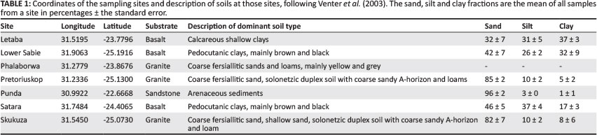
The Kruger National Park is situated in the north-east of South Africa between 30.9-32.0 °E and 22.3-25.5 °S. The park receives between 450 mm and 750 mm yr-1 of rain, most of which falls between October and March. Average temperatures are approximately 25 °C in summer and 20 °C in winter. Most of KNP is underlain by either basaltic rock that weathers into clay-rich soils or granitic rock that weathers into sandy soils. Both of these dominant parent materials are old: the basaltic rock was formed ~200 MA, whilst the granite was formed ~2050 MA (Venter et al. 2003). Seven dominant soil types from across the park (Venter et al. 2003) were sampled (Figure 1; Table 1). The sampled soil types cover approximately 65% of KNP.

Approach
Using a soil auger, samples were collected at three depths: at the top of the profile (0 cm - 10 cm), at the bottom (110 cm or degraded bedrock, whichever was shallower) and in the middle (Table 2). Soils were air dried and sieved in a 2 mm-aperture sieve to remove large roots and rocks. The proportion of rock with dimensions greater than 2 mm was generally negligible (< 3%).
Water retention curves
Soil moisture retention curves were derived empirically using an instrument that exploits the chilled-mirror technique (WP4T, Decagon Devices Inc., Pullman). A soil sample is inserted into the device and equilibrated with the headspace of a sealed chamber, so that the water potential of the air in the chamber is the same as the water potential of the sample. The point of condensation on a mirror is detected by shining a beam of light onto the mirror and recording its reflectance with a light sensor. At the point of condensation, the temperature of the mirror is recorded, allowing the water potential of the air, and therefore of the sample, to be calculated. The instrument measures the water potential with an accuracy of 0.05 MPa over the range of -0.1 MPa - -0.5 MPa and an accuracy of 0.1 MPa over the range of -0.5 MPa - -300 MPa. Therefore, it adequately covers the range relevant to plant growth. The water content of the sample at the time of measuring water potential is determined gravimetrically (i.e. it is weighed and reweighed after oven-drying at 60 °C to a constant weight). Since the relationship between water potential and water content is often hysteretic (affected by the initial state of the system), we constructed soil moisture retention curves from both drying and wetting soils.
Soil from each sampling location and depth was subdivided into 15 samples of 5 g - 6 g each. These samples were used to construct a single drying curve and a single wetting curve for each depth at each sampling location. For the drying curve, the samples were initially saturated with distilled water, sealed, and left to equilibrate overnight. Water potential and moisture content were then measured repeatedly as the samples air dried. A typical curve was completed within a day. For the wetting curve, incremental amounts of moisture were added to initially dry samples to achieve a range of saturation levels. Samples were then sealed and left to equilibrate overnight, after which the water potential and moisture content were measured.
Empirical models for the water retention curve are typically written to be solved for water content (see Assouline et al. [1998] for an overview). We fitted two widely used models, proposed by Van Genuchten (1980), and Fredlund and Xing (1994), which were rewritten to solve for water potential given a known water content using non-linear regression in R (R Core Team 2013). We compared the performance of these models to simpler power and exponential functions, which were fitted by maximising the likelihood using iterative methods (Plummer 2013). These functions were fitted to both the entire measured range of water potentials (0 MPa - -100 MPa) and to a subset that is relevant to plant growth (0 MPa - -8 MPa).
To assess the variability amongst sites of the same geology, we compared site-specific curves to curves for which the data were aggregated by geology. This was done for four levels of water content (0.03 g g-1, 0.05 g g-1, 0.1 g g-1 and 0.15 g g-1). For this analysis, soils from Punda, which are derived from quartzite (Venter et al. 2003), were included with granite-derived soils as they had a very similar texture.
Soil texture
Particle size affects the total surface area for a given mass or volume of soil, and therefore the shape of the water retention curve. To quantify sand, silt and clay fractions, the hydrometer method (Bouyoucos 1962) was used. For each sample, between 40 g and 50 g of soil was dispersed with an electrical mixer in 100 mL of a 5% sodium hexametaphosphate ([NaPO3]6) solution, in order to break down clay aggregates. This mixture was allowed to soak overnight and mixed again the following morning before being transferred to a 1 L cylinder filled up to 1 L with distilled water. Sediment was dispersed with a plunger and hydrometer readings were taken after 40 s and 6 h 52 min. Fractions were calculated as:


where H is the hydrometer reading at t seconds after inserting the hydrometer, and w is the sample weight in grams. Hydrometer readings were corrected for the added (NaPO3)6 by subtracting the hydrometer reading of a cylinder with 100 mL (NaPO3)6 solution filled up to 1 L with distilled water. The temperature was measured at the time of each hydrometer reading and 0.4 g L-1 of solute concentration was added to the hydrometer reading for every degree C above 20 °C (http://uwlab.soils.wisc.edu/files/procedures/particle_size.pdf).
Results
As expected, soils from the basalt substrate had a much higher clay content than soils from the granitic substrate (Table 1; Table 2).
The water potential and water content data is given in Online Appendix 1. The Fredlund and Xing model (1994) appeared to fit the data well, with R2 values > 0.99 for most curves. However, the confidence intervals on the parameter estimates could not be estimated using standard techniques, suggesting the parameters were not identifiable. In other words, multiple combinations of parameter values can result in an identical fit. This outcome is likely to be a symptom of over-parameterisation of the model. The Van Genuchten model (1980) did not converge well, also hinting at over-parameterisation. Therefore only results from the simpler power and exponential functions were reported.
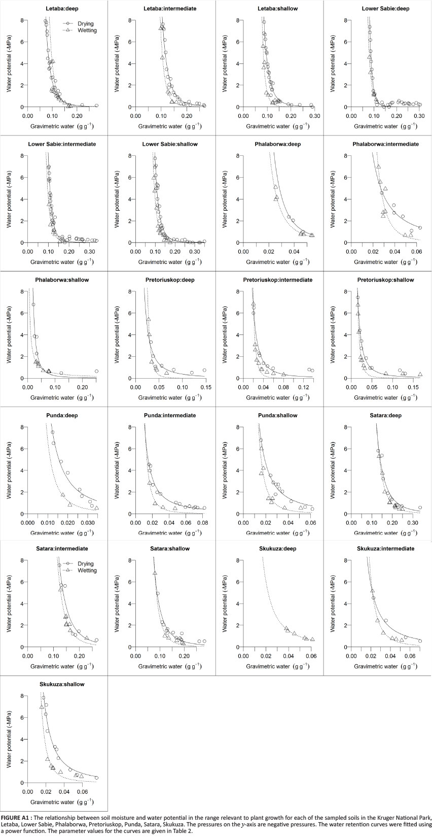
The best fit to individual curves in the -0.5 MPa - -8 MPa range was provided by a power function of the form (Table 2; Appendix 1):

where Ψ is water potential in MPa, Θ is gravimetric water content in g g-1, and a and c are estimated coefficients. For a given water content, water potentials from drying curves were generally lower than for wetting curves (Appendix 1).
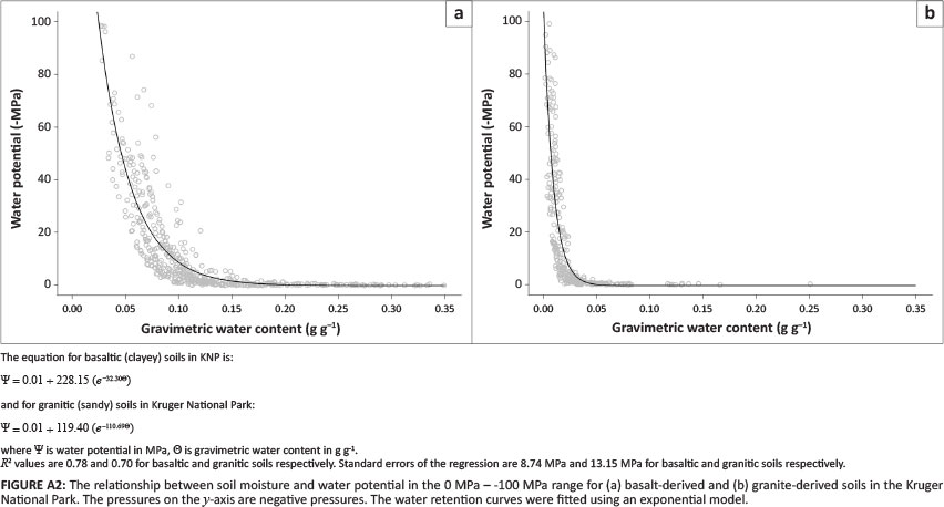
When combining data from all sites per geological substrate, the residuals of the power function fits showed systematic bias. An exponential model to describe the data aggregated by geology was therefore used. The exponential model fits these grouped data reasonably well in the -0.5 MPa - -8 MPa range: basalt R2 = 0.59; granite R2 = 0.66 (Figure 2; see Appendix 2 for 0 MPa - -100 MPa range). It should be noted that R2 values should be interpreted with caution in non-linear regression, and that the standard error of the regression (SER) is a better measure of goodness of fit: basalt SER = 1.42 MPa; granite SER = 1.13 MPa.
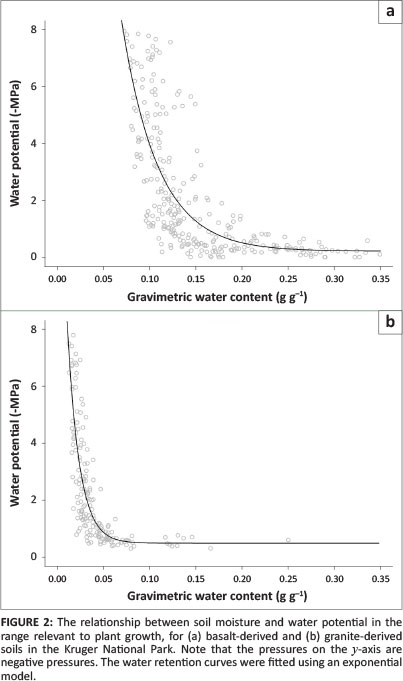
The equation to convert soil water content to water potential for basaltic (clayey) soils in the -0.5 MPa - -8 MPa range is:

For granitic (sandy) soils in the -0.5 MPa - -8 MPa range, the equation is:

To assess the accuracy of these geology-specific curves, we compared the range in water potential for four water contents (0.03, 0.05, 0.10 and 0.15), as predicted by the site-specific models to the predicted water potential, using the geology-specific curve (Figure 3). The geology-specific curves predicted water potentials close to the median value of site-specific curves, suggesting that they might be useful for modelling applications.

Discussion
Ecophysiological and hydrological interpretation of soil water content - an affordable measure of soil moisture - requires the use of pedo-transfer functions that transform water content into water potential. We generated such water retention curves with a WP4T instrument (Decagon Devices Inc., Pullman) using empirical data, and provided curves for common soil types in KNP, South Africa. A power function provided a good fit for individual samples, and, depending on the required accuracy, a single exponential function per geological substrate may be used. At low water contents (i.e. ~5% for granitic and ~15% for basaltic soils), water potentials estimated from our pedo-transfer functions begin to vary widely between sites, reflecting differences in clay content. Thus, researchers interested in precise estimates of soil water potentials in dry soils should use our site-specific functions. However, these water potentials are below the permanent wilting range (-1.5 MPa - -5 MPa; Figure 3) and represent small volumes of soil water.
Researchers using the equations provided here should take care to avoid several potential problems. First, our analyses relied on the chilled-mirror technique. This method is highly accurate in the dry range (-0.5 MPa - -300 MPa), but is less accurate in the wet range of soils (-0.001 MPa - -0.5 MPa). It should be noted that some crop species may become water limited at -0.03 MPa (Rodriquez-Iturbe & Porporato 2004). Second, the functions presented here are based on gravimetric soil water measurements, whilst some field sensors measure soil moisture volumetrically. To use the functions provided in this study, volumetric soil moisture should be divided by the bulk density of the soil. Bulk density in KNP varies with texture, spatially, and with soil depth (Wigley et al. 2013). When converting gravimetric or volumetric contents to water potentials, researchers should be aware of the potential role of coarse rock fragments. A soil sensor that provides volumetric water content in a rocky soil will underestimate soil water potentials because the volumetric sensor reports the water content of a volume comprised of both rock and soil.
In conclusion, the presented soil water retention curves will improve estimates of plant-available water from measurements of volumetric or gravimetric soil moisture in KNP and surrounding areas with similar geological substrates.
Acknowledgements
The authors would like to thank the management of the Kruger National Park for enabling this study. Ben Wigley kindly made bulk density data available; Tercia Strydom made equipment available; Alexander Zizka, Julia Fischer and Jenny Toivio assisted with data collection; and Stephen Doucette-Riise and his team collected soil samples. This study was funded by the Deutsche Forschungsgemeinschaft (DFG).
Competing interests
The authors declare that they have no financial or personal relationship(s) that may have inappropriately influenced them in writing this article.
Authors' contributions
R.B. (Goethe Universität Frankfurt) collected and analysed data, and wrote the article. A.K. (Utah State University) conceived the study and wrote the article. S.I.H. (University of Otago) analysed data and wrote the article.
References
Assouline, S., Tessier, D. & Bruand, A., 1998, 'A conceptual model of the soil water retention curve', Water Resources Research 34(2), 223-231. http://dx.doi.org/10.1029/97WR03039 [ Links ]
Baldocchi, D.D., Xu, L. & Kiang, N., 2004, 'How plant functional-type, weather, seasonal drought, and soil physical properties alter water and energy fluxes of an oak-grass savanna and an annual grassland', Agricultural and Forest Meteorology 123(1 & 2), 13-39. http://dx.doi.org/10.1016/j.agrformet.2003.11.006 [ Links ]
Bouma, J., 1989, 'Using soil survey data for quantitative land evaluation', in B.A. Stewart (ed.), Advances in Soil Science, pp. 177-213, Springer-Verlag, New York. http://dx.doi.org/10.1007/978-1-4612-3532-3_4 [ Links ]
Bouyoucos, G.J., 1962, 'Hydrometer Method Improved for Making Particle Size Analyses of Soils 1', Agronomy Journal 54(5), 464-465. http://dx.doi.org/10.2134/agronj1962.00021962005400050028x [ Links ]
Fredlund, D. & Xing, A., 1994, 'Equations for the soil-water characteristic curve', Canadian Geotechnical Journal 31(3), 521-532. http://dx.doi.org/10.1139/t94-061 [ Links ]
Lambers, H., Chapin III, F.S. & Pons, T.L., 2008, Plant Physiological Ecology, Springer, New York. http://dx.doi.org/10.1007/978-0-387-78341-3 [ Links ]
Plummer, M., 2013, JAGS - Just Another Gibbs Sampler, viewed 2013, from http://mcmc-jags.sourceforge.net/ [ Links ]
R Core Team, 2013, R: A Language and Environment for Statistical Computing, R Foundation for Statistical Computing, Vienna, Austria, viewed 2013, from http://www.R-project.org/ [ Links ]
Rodriquez-Iturbe, I. & Porporato, A., 2004, Ecohydrology of Water-Controlled Ecosystems: Soil Moisture and Plant Dynamics, Cambridge University Press, Cambridge. [ Links ]
Van Genuchten, M.T., 1980, 'A Closed-form Equation for Predicting the Hydraulic Conductivity of Unsaturated Soils', Soil Science Society of America Journal 44(5), 892-898. http://dx.doi.org/10.2136/sssaj1980.03615995004400050002x [ Links ]
Venter, F.J., Scholes, R.J. & Eckhardt, H.C., 2003, 'The abiotic template and its associated vegetation pattern', in J.T. du Toit, K.V. Rogers & H.C. Biggs (eds.), The Kruger Experience: Ecology and Management of Savanna Heterogeneity, pp. 83-129, Island Press, Washington DC. [ Links ]
Vogel, S., 2012, The Life of a Leaf, University of Chicago Press, Chicago. http://dx.doi.org/10.7208/chicago/9780226859422.001.0001 [ Links ]
Wigley, B.J., Coetsee, C., Hartshorn, A.S. & Bond, W.J, 2013, 'What do ecologists miss by not digging deep enough? Insights and methodological guidelines for assessing soil fertility status in ecological studies', Acta Oecologica 51, 17-27. http://dx.doi.org/10.1016/j.actao.2013.05.007 [ Links ]
 Correspondence:
Robert Buitenwerf
Altenhöferallee 1
60438 Frankfurt am Main
Germany
Email: buitenwerfrobert@hotmail.com
Received: 19 Mar. 2014
Accepted: 04 Aug. 2014
Published: 10 Nov. 2014
Appendix 1
Appendix 2

