RESEARCH ARTICLE

 

A new high-resolution geomagnetic field model for southern Africa

 

 

Amore E. Nel^I; Achim Morschhauser^II; Foteini Vervelidou^III; Jürgen Matzka^II

^ISouth African National Space Agency, Hermanus, South Africa
^IIGerman Research Centre for Geosciences, Potsdam, Germany
^IIIDepartment of Earth, Atmospheric and Planetary Sciences, Massachusetts Institute of Technology, Cambridge, Massachusetts, USA

Correspondence

 

 

---

ABSTRACT

Earth's magnetic field is a dynamic, changing phenomenon. The geomagnetic field consists of contributions from several sources, of which the main field originating in Earth's core makes up the bulk. On regional and local scales at Earth's surface, the lithospheric field can make a substantial contribution to the overall field and therefore needs to be considered in field models. A locally derived regional core field model, named HMOREG, has been shown to give accurate predictions of the southern African region. In this study, a new regional field model called the South African Regional Core and Crust model (SARCC) is introduced. This is the first time that a local lithospheric model, estimated by employing the revised spherical cap harmonic analysis modelling method, has been combined with the core component of CHAOS-6, a global field model. It is compared here with the existing regional field model as well as with global core field models. The SARCC model shows small-scale variations that are not present in the other three models. Including a lithospheric magnetic field component likely contributed to the better performance of the SARCC model when compared to other global and local field models. The SARCC model showed a 33% reduction in error compared to surface observations obtained from field surveys and INTERMAGNET stations in the Y component, and HMOREG showed a 7% reduction in error compared to the global field models. The new model can easily be updated with global geomagnetic models that incorporate the most recent, state-of-the-art core and magnetospheric field models.
SIGNIFICANCE:
Earth's magnetic field is an integral part of many current navigational methods in use. Updates of geomagnetic field models are required to ensure the accuracy of maps, navigation, and positioning information. The SARCC regional geomagnetic field model introduced here was compared with global geomagnetic field models, and the inclusion of a lithospheric magnetic field component likely contributed to the better performance of the SARCC model. This regional model of southern Africa could easily be updated on a regular basis, and used for high-resolution information on the Earth's magnetic field for the wider scientific community.

Keywords: geomagnetism, geomagnetic modelling, core field, crustal field, secular variation

---

 

 

 

Introduction

Earth is surrounded by its geomagnetic field, which protects us from the harmful effects of space weather.¹ The geomagnetic field also plays a role in navigation and mapping applications. The geomagnetic field originates primarily from the core due to the dynamo process occurring therein. Another geomagnetic field source is the magnetised part of Earth's crust.^2,3 This magnetic field component is known as the lithospheric magnetic field. The core field shows temporal variability on timescales of 1 year and longer⁴, while the lithospheric field is, to a good approximation, time-invariant. Another difference between these two components of the geomagnetic field is spatial variation.² The core field dominates over large wavelengths (several thousands of kilometres) while the lithospheric field dominates over short (less than 500 km) wavelengths of the observed geomagnetic field. Geomagnetic field models can be expanded in spherical harmonic functions, solving the Laplace equation in spherical coordinates.⁴ There is also an external field, formed by the interaction of the solar wind with the Earth's magnetosphere, that makes up the external contribution to the geomagnetic field from near-Earth current systems. This field has time scales in the order of seconds to days, much less than secular variation.³

The southern African region is known for its temporally and spatially highly variable geomagnetic field.^4,5 Due to the small-scale variations, the current available global field models are unable to describe this region accurately. A model called Southern African Model made of Splines (SAMS), using harmonic splines, was derived for this region, which consisted only of a core component.³ In this study, core and lithospheric components were combined to create a new regional model. The lithospheric field component was obtained by employing a spherical harmonic degree of 16 and larger in the model. This component was derived by using ground measurements from repeat stations, which enabled the addition of small-scale spatial variations in the model predictions. For the core component, we used spherical harmonic degrees from 1 to 15. Combining both contributions into one model can improve the accuracy of the magnetic field model predictions. Two global field models, the CHAOS-7 and the IGRF-13 model, which will be discussed in more detail in the sections to follow, were compared with the two southern African regional field models, HMOREG and SARCC.

 

Global field models

IGRF-13

The International Geomagnetic Reference Field (IGRF) is a spherical harmonic model used to describe the large-scale main (core) field globally and is updated every 5 years using observatory and satellite mission data sets.⁶ The 13th generation used in this study covers the period from 1900 to 2025.⁷ The current version was expanded to a maximum spherical harmonic degree of 13. Neither this model nor the CHAOS model incorporates field survey data from southern Africa.

CHAOS-6

CHAOS is a series of core field models derived by the Technical University of Denmark.⁸ Along with the basic 0rsted, CHAMP and SAC-C satellite mission data sets used in the earlier CHAOS models, CHAOS-6 also uses monthly means derived from the hourly mean values of 160 ground observatory magnetic measurements and over 2 years of Swarm data available up until March 2016.⁹ CHAOS-6 includes along-track differences between two Swarm satellites, Alpha and Charlie. It covers the epoch from 1997 to 2018.⁸ Only the internal magnetic field contributions, the core and crust components, were used in this study.

CHAOS-7

CHAOS-7 is the latest of the CHAOS series and was released at the end of 2019; it includes both core and crustal components. The model is based on 0rsted, CHAMP SACC, Cryosat2, and Swarm satellite data, as well as ground geomagnetic observatory data.

 

Regional field models

HMOREG

The Hermanus Magnetic Observatory (34°25.5' S, 19°13.5' E) was established in 1941 and today falls under the South African National Space Agency (SANSA).¹⁰ Between 1960 and 2005 there was an undertaking to establish other magnetic observatories in southern Africa. A site was identified outside Tsumeb (19°°12' S, 1735' E) in Namibia in 1964 on the premises of a permanent ionospheric observation station of the Max Planck Institut für Aeronomie. Another was established at Hartebeesthoek (25°°52.9' S, 27°42.4' E) in 1972. These, along with the observatory at Hermanus, are members of the INTERMAGNET network.¹¹

Since 2005, two sets of 20 repeat stations have been measured bi-annually in survey campaigns across southern Africa, which include South Africa, Namibia, Zimbabwe, and Botswana.¹⁰ Along with the continuous recording output of the three aforementioned INTERMAGNET stations, these data were used to derive a polynomial-based core field regional model. This mathematical model was derived using third-order polynomials with 10 statistically significant coefficients:

where p refers to the main field components (F, H, D, Z), X = 26° latitude, and Y = 24° longitude. The coefficients A-J were estimated from the field survey data using a least-squares fit for each separate component. This model is referred to as HMOREG. In this study, only input grid points that fell within the boundaries defined by the location of the outermost repeat stations were considered. This model is updated annually using the latest field surveys. Field survey locations for 2016 are shown in Figure 1. Since 2016, the number of repeat stations has been reduced to 19.

SARCC

The latest model for southern Africa that we describe in this paper is a novel coupling of the CHAOS-6 core model (for spherical harmonic degrees 1 to 15) and the lithospheric field model of Vervelidou et al.¹² The combined model is referred to as the South African Regional Core and Crust (SARCC) model henceforth. It accepts as input an epoch, and the altitude and geodetic coordinates of whichever grid points are desired. As output, it calculates the north, east and downward components of the magnetic field as well as the magnetic field declination. The model only accepts grid points within the lithospheric model of Vervelidou et al.¹² The SARCC model can be updated by adding future global field model versions instead of the CHAOS-6 model.

The SARCC is a high-resolution model based on satellite, near-surface, and ground magnetic field measurements. It is parameterised by the revised spherical cap harmonic analysis (R-SCHA) modelling method. The latter is a regional analysis technique used to obtain magnetic field measurements at different altitudes.¹³ The lithospheric magnetic field is modelled inside the volume of a spherical cone over southern Africa with a half-angle aperture of θ₀ =15 centred at a geocentric longitude of 22.5° E and latitude of 25° S, excluding a thin ring of 0.1° from the cap's volume using the R-SCHA modelling method. The spherical harmonic degree starts at 16 (which corresponds to wavelengths of about 2500 km) and goes up to degree and order 1400. It can predict the geomagnetic field at altitudes ranging from 0 to 500 km. The R-SCHA result relies on CHAMP and Swarm satellite magnetic field measurements and on a version of the World Digital Magnetic Anomaly Map (WDMAM) that relies on aeromagnetic and marine measurements taken over southern Africa since 1970, and it has a spatial resolution of 0.1°. The model also includes data from repeat station measurements conducted annually throughout 2005-2009. Finally, the annual means of three geomagnetic observatories - Hermanus and Hartebeesthoek in South Africa and Tsumeb in Namibia (Figure 1) - were also part of the input data set.

 

Methods

Comparison methodology

The global IGRF-13 and CHAOS-7 models, and the two southern African regional field models SARCC and HMOREG, were compared with each other. It is important to note that IGRF-13 and HMOREG do not take into account the lithospheric field, whereas SARCC and CHAOS-7 do.

The model predictions were also compared to the results of the repeat station surveys. As mentioned in the section describing the HMOREG regional field model, surveys have been conducted at several repeat stations across southern Africa since 2000.

These surveys take place between middle September to middle December and are split between two fieldwork legs: one leg covers the stations on the eastern side of South Africa and the other covers the western side. Each repeat station is marked by concrete beacons, which ensures that the location of observation points stays constant for successive surveys. Geomagnetic field observations are done in the early evening and early morning, with the variometer operating continuously during the night.¹⁴ The data are augmented by standard observatory annual means and centred in the middle of each year. The reduction methodology is the same for both the eastern and western leg data sets. The data are not corrected for external or lithospheric signals.¹⁵

Statistical method

In this study, the field surveys from 2015.5, 2016.5, 2017.5, and 2018.5 epochs were combined with recordings from four INTERMAGNET observatories: Hermanus (HER), Hartebeesthoek (HBK), Keetmanshoop (KMH), and Tsumeb (TSU). These values were then compared with the values predicted by the four models introduced earlier.

For each of the four epochs considered in this study, the magnetic field components X, Y, Z (which represent the three orthogonal component field directions for local geodetic northward, eastward, and vertically down, respectively) and the declination D were determined at the survey location points using the four models - SARCC, HMOREG, CHAOS-7, and IGRF-13. The total number of locations was 40 for 2015.5, 22 for 2016.5, 24 for 2017.5, and 22 for 2018.5. Only the 19 points common to all field surveys were used for the comparison. From this, the mean difference was determined for each component of each model by comparison with the field survey data over all the years. To get an idea of each model's error distribution characteristics, the standard deviation and skewness were estimated from the average value over all available years. Lastly, the secular variation over all available data sets was determined using each model and compared with the field survey results. Secular variation at time t was taken as the differences of the X, Y, and Z values at time t + 6 months and t - 6 months.

 

Results and discussion

For the sake of comparison, a 0.2° resolution grid for the predicted Y component over southern Africa is shown for each model in Figure 2 within the borders of each respective model. The SARCC predicted grid in the top right figure shows small-scale variations and gives more information about local anomalies on the surface. The lithospheric model predictions are also shown separately for the X, Y, and Z components at Earth's mean reference radius using the SARCC model for 2018.5 in Figure 3. The SARCC model lithospheric field signal includes many fine-scaled magnetic field features at Earth's mean reference radius that are not present in the other models.

Comparisons were made between differences at every field survey location and INTERMAGNET observatories. A visual representation of these differences for the Y component (in nT) is shown in Figure 4 for all available years. The standard error of the mean (SEM) is calculated by Equation 2:

where σ is the standard deviation and n is the sample size. SEM was calculated as 6.8 nT, 9.4 nT 10.1 nT, and 10.1 nT for SARCC, HMOREG, IGRF-13, and CHAOS-7, respectively. The SEM gives an indication of how much discrepancy is likely in the sample mean compared with the population mean. In this case, the population mean was the mean derived from the respective model outputs, and the sample mean was calculated from the field survey data. SARCC shows the least amount of difference between field survey measurements and prediction, with a ~32.7% reduction in error compared to the global field models. HMOREG also shows smaller differences compared to the global field models IGRF-13 and CHAOS-7, with a ~6.9% reduction in error. Similar prediction performance is seen for the X component. For the X component, the SEM was calculated as 7.0 nT, 8.8 nT, 10.8 nT, and 12.2 nT for SARCC, HMOREG, IGRF-13, and CHAOS-7, respectively, which is a 39.1% and 23.5% reduction in error for SARCC and HMOREG, respectively, when compared to global field models. For the Z component, the SEM was calculated as 12.4 nT, 21.4 nT, 22.8 nT, and 18.8 nT for SARCC, HMOREG, IGRF-13, and CHAOS-7, which gave a 40.4% reduction in error and a 2.9% increase in error for SARCC and HMOREG, respectively, when compared to global field models. Of all the models, the SARCC shows the least amount of difference between prediction and field survey measurements. The histograms of the differences between the 19 repeat station measurements and the model predictions for all available years are shown in Figure 5 for the Y component, with the mean and variance indicated in the legends of each plot. The standard deviation (σ) of the SARCC is lower than those of the other three models for all components (Table 1).

Results of the statistical comparisons of the differences between the measured and modelled components for 2015.5-2018.5 are also shown in Table 1. The standard deviation measures the variability of the data set to the mean. The standard deviation does give an indication of the predictive abilities of each model, but given the size of the area from which these statistical measurements are derived, and considering local, temporal, magnetic anomalies, using the standard deviation for a baseline correction could cause an erroneous result. The SARCC model standard deviations are, on average, 39%, 33%, 43%, and 32% lower than the global field models for X, Y, Z, and declination, respectively. Thus, SARCC shows the least deviation for all examples in all components. HMOREG's performance varies, as can be seen in Figure 5 and Table 1. HMOREG's standard deviation is on average 24%, 7%, and 9% lower than the global field models for X, Y and declination. HMOREG's standard deviation for the Z component is 4% more than that for the global field models. The standard deviation for HMOREG is lower for the X and Y components, as well as declination, compared to those of the global field models.

The skewness of a data set is defined as the distortion or deviation from a normal distribution. The distribution can be negatively or positively skewed, but here we refer only to the absolute skewness. If skewness is less than 0.5, the distribution is approximately symmetrical; if the skewness is between 0.5 and 1, it is moderately skewed; and if the skewness is greater than 1, the distribution is described as highly skewed. The SARCc's X component is moderately skewed, the Y component highly skewed, and the Z component approximately symmetrical. HMOREG's X and Y components are approximately symmetrical, and the Z component is moderately skewed.

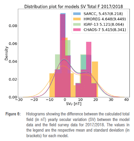
The calculated secular variation for the total field for 2017/2018 is shown in Figure 6. This plot shows the difference between the secular variation measured during field surveys (referred to the middle of the respective year as described in the 'Statistical method' section), and the values determined by the respective models. All models show similar outputs, with the double peak visible in the total field histogram showing a deviation between the model predictions and field survey measurements. The field survey data were measured and collected in two phases: an east leg and a west leg. The total field values of the repeat stations for all available years are shown in Supplementary table 1. From these values, the secular variation is derived and shown in columns SV1516, SV1617, and SV1718. The locations that fall under the west leg are highlighted in yellow, and the locations for the east leg are in blue. From the average secular variation values (in rows labelled 'AVG W' and 'AVG E') in Supplementary table 2, it is clear that there is a significant increase in secular variation strength moving from east to west. Models in this study have been shown to overestimate the west leg data set and underestimate the east leg data set, albeit to a lesser extent than the ground observatory data. The data reduction methodologies used for the repeat stations are the same for both data sets, which leads to the conclusion that this double peak is likely because of the presence of the South Atlantic Anomaly and the most recent geomagnetic jerk, and the cause of this spatial gradient observed over southern Africa. The South Atlantic Anomaly is an area over the Atlantic Ocean where there is a significant depletion of magnetic field strength, and partially overlaps southern Africa. Supplementary table 2 shows the calculated CHAOS values for secular variation for the same times and locations as the repeat stations; these values were used to cross-correlate the results shown in Supplementary table 1. Although there was also a predicted increase in secular variation, thus picking up the magnetic field gradient due to the South Atlantic Anomaly, the CHAOS model does not pick it up as intensely as the ground observatory measurements.

 

 

Rapid secular variation pulses, or jerks, have been identified across the globe. Previous studies pertaining to the southern African region have noted its rapid changes in secular variation pattern.^16-18 The 2014 jerk was observed in southern Africa and was analysed by Kotzé¹⁹ using data from four observatories located at Hermanus, Hartebeesthoek, Keetmanshoop and Tsumeb. It was found that the data from all four of these observatories showed strong individual characteristics. These rapid changes in magnetic field cannot always be predicted by global geomagnetic field models¹⁶ - an observation also seen in this study.

Using the CHAOS secular variation model, Mandea et al.¹⁷ also showed that southern Africa is prone to rapidly changing secular variation. It was also clear from their study that the secular variation was more intense on the western side of South Africa than on the astern side. This finding can also be seen from the latest IGRF model output²⁰ (see Supplementary figure 1).

It should also be noted that jerks are not always observed simultaneously in all geomagnetic field components at a particular observatory¹⁷, which should be taken into consideration when interpreting the results of this study where the secular variation of the total field is shown.

 

Conclusions

When looking at the total data set spanning over 4 years, both local field models (SARCC and HMOREG) deviated less from the mean than the global field models (CHAOS-7 and IGRF-13). Overall, SARCC showed a higher reduction in error than HMOREG and HMOREG showed a considerably lower skewness than SARCC.

When interpreting the secular variation results from this study, both the gradient of the secular variation strength observed over southern Africa (increasing in intensity from east to west) and the diverseness of the secular variation strength should be considered. The former is due to the presence of the South Atlantic Anomaly and is the cause of the spatial variability observed in this region. The latter is possibly due to the inhomogeneous occurrence of jerks at different locations, as well as the current limited prediction capabilities of global field models for rapid secular variation events.^5,10,16 A complete analysis and interpretation of this topic is beyond the scope of this paper and will be part of future work.

The new regional SARCC model consists of a core field from the CHAOS-6 global field model and a high-resolution lithospheric field component derived from several input data sets including regional field surveys. The novelty of this model is the inclusion of ground measurements from repeat station data for the lithospheric component, which enables the inclusion of small-scale spatial variations in the region usually not possible by global field models.

This model can be updated to include the latest version, CHAOS-7. It compares well with field survey data taken during four campaigns from 2015 to 2018, specifically when looking at the standard deviation for each respective component, as well as the distribution of each component. The SARCC showed on average a 33% reduction in error compared to the global field models. This is likely due to the inclusion of a lithospheric magnetic field component in the model, which includes regionally dependent, small-scale variations with a much weaker signal than the core component.¹⁶ It is easy to produce updates for this model, and because of the availability of regional field surveys in southern Africa, the model can regularly be evaluated for accuracy.

 

Acknowledgements

We thank the South African National Research Foundation and the South African National Space Agency for funding and Dr Nahayo (SANSA) for providing the field survey data used in this study.

Competing interests

We have no competing interests to declare.

Authors' contributions

A.E.N.: Methodology; data analysis; validation; writing - the initial draft; writing - revisions. A.M.: Conceptualisation. F.V.: Conceptualisation; validation. J.M.: Conceptualisation.

 

References

1. Mandea M, Chambodut A. Geomagnetic field processes and their implications for space weather. Surv Geophys. 2020;41:1611-1627. https://doi.org/10-1007/s10712-020-09598-1        [ Links ]

2. Backus G, Parker R, Constable C. Foundations of geomagnetism. Cambridge: Cambridge University Press; 1996.         [ Links ]

3. Geese A, Mandea M, Lesur V, Hayn M. Regional modelling of the southern African geomagnetic field using harmonic splines. Geophys J Int. 2010;181:1329-1342. https://doi.org/10.1111/j.1365-246X.2010.04575.x        [ Links ]

4. Langel R, Hinze W. The magnetic field of the earth's lithosphere: The satellite perspective. Cambridge: Cambridge University Press; 2020. https://doi.org/10.1017/CBO9780511629549        [ Links ]

5. Mandea M, Holme R, Pais A, Pinheiro K, Jackson A, Verbanac G. Geomagnetic jerks: Rapid core field variations and core dynamics. Space Sci Rev. 2010;155:147-175. https://doi.org/10.1007/s11214-010-9663-x        [ Links ]

6. Thébault E, Finlay CC, Beggan CD, Alken P, Aubert J. Barrois O, et al. International geomagnetic reference field: The 12th generation. Earth Planet Sp. 2015;67, Art. #79. https://doi.org/10.1186/s40623-015-0228-9        [ Links ]

7. Alken P International Geomagnetic Reference Field [webpage on the Internet]. No date [updated 2019 Dec 19; cited 2020 Feb 24]. Available from: www.ngdc.noaa.gov/IAGA/vmod/igrf.html        [ Links ]

8. Olsen N, Lühr H, Finlay CC, Sabaka TJ, Michaelis I, Rauberg J, et al. The CHAOS-4 geomagnetic field model. Geophys J Int. 2014;197(2):815-827. https://doi.org/10.1093/gji/ggu033        [ Links ]

9. Finlay CC, Olsen N, Kotsiaros S, Gillet N, Clausen L. Recent geomagnetic secular variation from Swarm and ground observatories as estimated in the CHAOS-6 geomagnetic field model. Earth Planet Sp. 2016;68, Art. #112. https://doi.org/10.1186/s40623-016-0486-1        [ Links ]

10. Kotzé PB. Hermanus magnetic observatory: A historical perspective of geomagnetism in southern Africa. Hist Geo Space Sci. 2018;9:125-131. https://doi.org/10.5194/hgss-9-125-2018        [ Links ]

11. St-Louis B. INTERMAGNET Technical reference manual [webpage on the Internet]. c2012 [cited 2020 Jul]. Available from: https://intermagnet.org/docs/Technical-Manual/technical_manual.pdf        [ Links ]

12. Vervelidou F, Thébault E, Korte M. A high-resolution lithospheric magnetic field model over southern Africa based on a joint inversion of CHAMP, Swarm, WDMAM, and ground magnetic field data. J Geophys Res Solid Earth. 2018;9:897-910. https://doi.org/10.5194/se-9-897-2018        [ Links ]

13. Thébault E. Global lithospheric magnetic field modelling by successive regional analysis. Earth Planet Sp. 2006;58:485-495. https://doi.org/10.1186/BF03351944        [ Links ]

14. Nahayo E, Kotzé PB, Korte M, Webb SJ. A harmonic spline magnetic main field model for southern Africa combining ground and satellite data to describe the evolution of the south Atlantic anomaly in this region between 2005 and 2010. Earth Planet Sp. 2018;70, Art. #30. https://doi.org/10.1186/s40623-018-0796-6        [ Links ]

15. Kotzé PB, Korte M, Mandea M. Polynomial modelling of southern African secular variation observations since 2005. Data Sci J. 2011;10. https://doi.org/10.2481/dsj.IAGA-16        [ Links ]

16. Kotzé PB, Korte M. Morphology of the southern African geomagetic field derived from observatory and repeat station survey observations: 20052014. Earth Planet Sp. 2016;68, Art. #23. https://doi.org/10.1186/s40623-016-0403-7        [ Links ]

17. Kotzé PB. The time-varying geomagnetic field of southern Africa. Earth Planet Sp. 2003;55:111-116. https://doi.org/10.1186/BF03351738        [ Links ]

18. Kotzé PB. The 2014 geomagnetic jerk as observed by southern African magnetic observatories. Earth Planet Sp. 2017;69, Art. #17. https://doi.org/10.1186/s40623-017-0605-7        [ Links ]

19. Kotzé PB. Statistical evaluation of global geomagnetic field models over southern Africa during 2015. Earth Planet Sp. 2017;69, Art. #84. https://doi.org/10.1186/s40623-017-0670-y        [ Links ]

20. Alken P Thébault E, Beggan CD, Amit H, Aubert J, Baerenzung J, et al. International Geomagnetic Reference Field: The thirteenth generation. Earth Planet Sp. 2021;73, Art. #49. https://doi.org/10.1186/s40623-020-01288-x        [ Links ]

 

 

Correspondence:
Amoré Nel
Email: anel@sansa.org.za

Received: 09 Aug. 2021
Revised: 01 Aug. 2023
Accepted: 11 Oct. 2023
Published: 30 Jan. 2024

 

 

Editor: Michael Inggs
Funding: South African National Research Foundation, South African National Space Agency

 

 

Supplementary Data

The supplementary data is available in pdf: [Supplementary data]