


Services on Demand
Article
 English (pdf)
 Article in xml format
 Article references
Indicators

Related links
-
 Cited by Google
 -
 Similars in Google
Share

 Permalink
South African Journal of Science
On-line version ISSN 1996-7489
Print version ISSN 0038-2353
S. Afr. j. sci. vol.118 n.3-4 Pretoria Mar./Apr. 2022
http://dx.doi.org/10.17159/sajs.2022/11933
RESEARCH ARTICLE
Determining safe retirement withdrawal rates using forward-looking distributions
Vaughan van AppelI, II; Eben MaréIII
IDepartment of Statistics, University of Johannesburg, Johannesburg, South Africa
IIDepartment of Actuarial Science, University of Pretoria, Pretoria, South Africa
IIIDepartment of Mathematics and Applied Mathematics, University of Pretoria, Pretoria, South Africa
ABSTRACT
An important topic for retirees is determining how much they can safely withdraw from their retirement savings: draw too much from their retirement fund and risk outliving their retirement savings, or draw too little and live below their means. For retirees to decide on the appropriate withdrawal rate, retirees need to have the tools available to decide on their spending rates. There are many factors that influence withdrawal rates, such as initial wealth, asset allocations, age, life expectancy, and risk tolerances. The topic of safe withdrawal rates aims to optimise spending rates while minimising the risk of running out of retirement savings. The focus of this study was on using forward-looking moments of the risk-neutral and real-world asset distributions in determining safe withdrawal rates for South African retirees. The use of forward-looking information, typically derived from traded derivative securities (rather than historical data), is essential in optimising safe withdrawal rates for retirees. In particular, we extracted the forward-looking risk-neutral and real-world distributions from option prices on the South African Top 40 index, and used the moments of the distributions as a signal in a simple tactical asset allocation framework. That is, when we expect the growth asset to decrease in value, we hold cash (or short the asset) and, alternatively, when we expect the growth asset to increase in value, we hold the growth asset for the period. Using this approach, we found that we can sustain withdrawal rates of up to 7% compared to the commonly quoted 4% safe withdrawal rate obtained by historical simulations.
SIGNIFICANCE:
• Through this paper, we aim to create further awareness on safe retirement spending rates. It is important that retirees are guided through this process with the correct knowledge of the risk and return of asset classes.
• Using forward-looking information allows for a more realistic modelling of portfolio returns, which allows for the possibility of better modelling of safe withdrawal rates.
• We show that using the moments of the forward-looking distributions in a simple tactical asset allocation framework yielded superior portfolio returns to a fixed asset allocation structure.
Keywords: safe withdrawal rates, forward-looking distributions, tactical asset allocation
Introduction
Studies on safe retirement spending rates typically draw information from historical data.1-5 A prime example of such a study is the commonly quoted '4% safe withdrawal rate' published in Cooley et al.1, where the authors used historical data over the period 1926 to 1995 to assess safe spending rates for retirees. The assumptions made in these studies are that the statistical properties of historical returns remain stable over time. However, it is known that historical (backward-looking) returns do not necessary predict future returns. Furthermore, in these studies, the authors assume a fixed asset allocation and a constant spending rate. Both assumptions are heavily criticised in the literature.5-7 People nowadays are living longer and face a further 20 to 30 years of life with substantial probability after retirement.8-10 Van Appel et al.5 demonstrated in an empirical study, using historical data, that for higher spending rates, a higher allocation in growth assets is needed. Even then, the portfolio is unlikely to be successful over a 30-year period (representing a typical post-retirement investment cycle). Ideally, a retiree would like to draw as much as possible, with a low probability of depleting the fund before their duration of life, or 30 years.
An important part of modelling is to generate scenarios for financial practitioners. In particular, it is important that these scenarios are as close as possible to the true representation of what could happen. In extension of the work presented by Cooley et al.1,2, Bengen3, and Maré4, the focus of this study was to improve the modelling of safe retirement spending rates by using forward-looking information rather than historical information. Many large financial institutions regularly estimate forward-looking distributions from option prices in order to gain insights into the weights investors place on different future asset prices.11,12 Therefore, modelling retirement withdrawal rates using forward-looking information should provide a more realistic assessment of safe withdrawal rates. The main advantage of using forward-looking information is that it allows for the implementation of a tactical asset allocation framework instead of a fixed asset allocation structure that is used in the literature. This allows the portfolio to potentially achieve higher asset returns, which increases the success rates of retirement portfolios. In particular, we would like to be invested in the risky (or growth) asset when the return is expected to be favourable to the portfolio. To assess when returns will be favourable, forward-looking information should be used rather than historical data. We thereby show that models based on historical data do not provide a true representation of modelling retirement portfolio success rates optimally.
Methodology
Typically, safe retirement withdrawal rates are analysed by using models based on historical data and Monte Carlo simulation.1-6,13,14 In particular, Scott13 studied the impact that a portfolio's rate of return has on safe withdrawal rates, and found that increasing the rate of return, by increasing the equity allocation, in the retirement portfolio drastically increases safe withdrawal rates. However, this comes with higher variability in returns (or risk).5 Therefore, the aim of this section is to use forward-looking information in a tactical asset allocation framework to maximise portfolio returns and reduce the variability in returns.
Extracting forward-looking return distributions
A European-style call option is a contract that gives the holder the right (but not the obligation) to purchase a prescribed asset from the writer, for a prescribed price at a prescribed time, in the future. The price of the contract is determined by its expected future pay-off, under the risk-neutral measure, discounted by the risk-free interest rate:
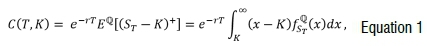
where T denotes the time to expiry (tenor), K the predetermined asset price (strike price), rlhe risk-free interest rate, STlhe asset price at expiry and  the risk-neutral probability density function of the future asset price. These options are typically traded on a number of official exchanges. Because the option pay-off extends out in time, option prices capture some market sentiment.15-20 This is known as forward-looking information.
The forward-looking risk-neutral probability density function,  , is easily extracted from market option prices by taking the second partial derivative with respect to the strike of a European call option as follows (see, Breeden and Litzenberger21):
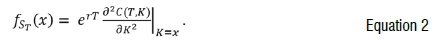
However, option price data are normally sparse and noisy, especially in South Africa. Therefore, to estimate the forward-looking risk-neutral density function in Equation 2, one typically first needs to interpolate and extrapolate call option prices over a dense strike range.22-25 It is practically more desirable to interpolate and extrapolate over the implied volatilities rather than the call option prices, where the implied volatilities can be obtained by the Black-Scholes option pricing formula.18 That is, the Black-Scholes option pricing formula is simply used to move between prices and implied volatilities. In this paper, we used the stochastic volatility inspired model, proposed by Gatheral24, to interpolate and extrapolate the implied volatility over a 50-150% moneyness range25. Thereafter, we numerically approximated the risk-neutral distribution by taking the second difference along the interpolate and extrapolate call option price at tenor t.11,18,26
Consequently, the moments of the distribution have become powerful in analysing and forecasting future returns.15,18,27 The risk-neutral distribution differs from the real-world distribution in that the risk-neutral distribution's expected return is the risk-free rate as investors are risk-neutral under this measure. However, investors are typically risk-averse and therefore require a premium for taking on the risk. That is, the risk-neutral measure is the real-world measure with the risk premium removed. For forecasting future asset returns, the real-world measure is, therefore, preferred.12,28 The risk premium is not directly observed and, therefore, obtaining the real-world measure normally involves additional assumptions on a utility function of terminal wealth and using historical data.18,29-31
Recently, Ross32 proposed the recovery theorem, which is an alternative method of extracting a real-world distribution from the risk-neutral matrix of a Markovian state variable, i.e.:

where t represents the option tenor. In this study, we numerically discretise Equation 3 over n=51 return states, in total spanning the moneyness range 50-150%, which is placed every 2% symmetrically around the moneyness of 100% to obtain the (mx n) state price matrix, S.32This is done by numerically integrating Equation 3 over the discrete grid for each of the 51 states.33 In essence, the discretised S(t,n) represents the price of an Arrow-Debreu security that agrees to pay one unit of currency if state j is reached at time t and zero in all other states.
In contrast, the recovery theorem does not make use of historical returns, but rather makes assumptions about market restrictions.32 This makes the recovery theorem a desirable candidate for extracting the real-world probabilities, particularly for new assets on the market, where large historical data sets do not exist. Under the assumption that transition state prices are time-homogeneous, the transition probability, P), of moving from state i to state j in one period is given as:

which can be estimated by solving the linear system of equations (see, for example, Ross32, Audrino et al.15, Van Appel and Maré25):
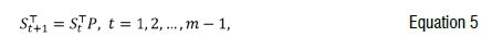
where P denotes the one-period risk-neutral transition probability matrix. Intuitively, P represents the richer set of probabilities of moving from all hypothetical initial states to all hypothetical future states, where Equation 3 only represents the probabilities of moving from the single known current state to all future states.34 Assuming no arbitrage, irreducibility of the transition matrix P, and that the pricing matrix is generated by a transition independent kernel, then under Ross's framework there exists a unique positive pricing kernel defined as the ratio price per unit probability:
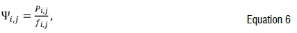
where represents the pricing kernel, and the real-world transition probability of moving from state to state in one period. In essence, Ross32 then estimates the two unknowns, namely the real-world probabilities and pricing kernel in Equation 6 using the Perron-Frobenius theorem.
To test the usability and practicality of the real-world distribution obtained by the recovery theorem in determining safe withdrawal rates, we next use the forward-looking forecasted moments in a simple tactical asset allocation framework to obtain higher returns than a model based purely on historical data with a fixed asset allocation. Furthermore, we also consider a hedging strategy by buying and selling put and call options, respectively.
Tactical asset allocation
In this section, we use the extracted forward-looking risk-neutral and real-world return distributions to forecast movements in the underlying asset returns. We extracted the forward-looking risk-neutral and real-world distributions, at the start of each month, from market-observed option prices quoted on the FTSE/JSE Top 40 index (Top40) over the period August 1996 to January 2018 (sourced from the South African FTSE/JSE), giving a total of 259 forecast months (or 259 one-month forecast distributions). The Top40 index was used as it is a key market factor in South Africa and, along with the exchange-traded derivatives on this asset, is one of the most liquid in the South African market. Furthermore, the duration of the sample (i.e. 21.5 years) would typically embrace at least three South African business cycles.35 Thereafter, we use the extracted risk-neutral and real-world moments in a simple tactical asset allocation framework to obtain higher returns for the portfolio.
Investors are normally in search of higher returns, skewness and kurtosis, and lower volatility. Therefore, as outlined in Audrino et al.15 and Flint and Maré16, we carried out a simple tactical asset allocation, where we hold the Top40 for the full month when the forecasted moments (mean, skewness, and kurtosis) are higher than the previous month's forecast, or when the forecasted volatility is lower than the previous month's forecast. Because trading occurs once a month, there are a limited number of trades, resulting in negligible transactional costs (transactional costs are normally around 2 basis points). In particular, we found that trading costs decreased yearly returns on average by no more than 0.2%. For completeness, all results based on the tactical asset allocation framework reported in this paper include transaction costs.
Lastly, we also considered a fixed asset allocation framework by incorporating a hedging strategy, where instead of selling the Top40 in the tactical asset allocation framework, we protect the portfolio against large losses by buying put options. This strategy involves purchasing put options with 6% out the money (OTM) strike with a 30% participation rate. Because put options are expensive, we offset the cost by selling call options with 1% OTM strike with a 30% participation rate. Because we use observed market-quoted prices, these parameter values were chosen to yield stable and desirable results. That is, our index portfolio value evolves as follows:
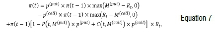
where π(ί) represents the portfolio value at time t, p()represents the participation rates, M()the moneyness rate, Rtthe asset return, and P(t,M(put))the market-quoted put option price.
The cumulative portfolio value over the period August 1996 to January 2018 for the simple tactical asset allocation framework using the moments of the risk-neutral and real-world distributions is shown in Figure 1a and Figure 1b, respectively, if one unit of currency was invested in the Top40 in August 1996.
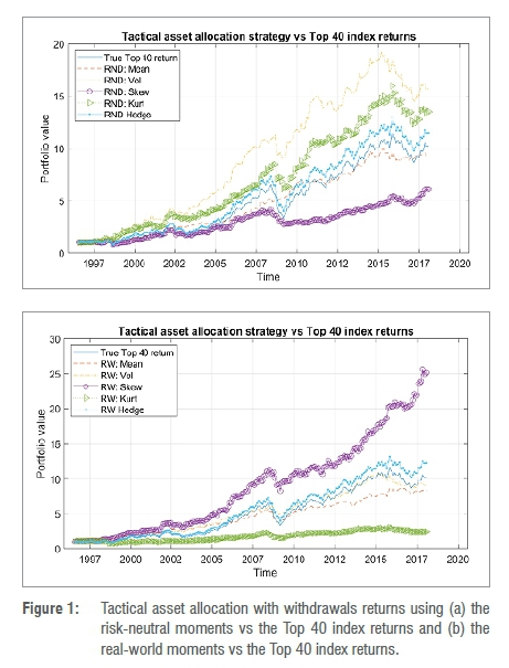
Figure 1a shows the portfolio using the forecasted risk-neutral volatility in returns as the signal in the tactical asset allocation framework yielded the best results. The trading strategy using the risk-neutral kurtosis also outperformed the Top40, while the trading strategy using the risk-neutral mean return yielded similar results to the Top40. The skewness yielded similar results to around 2005, but thereafter yielded poor results. In Figure 1b, the real-world skewness in the simple tactical asset allocation framework yielded the best results, while the volatility and mean yielded similar returns to the Top40, and the kurtosis yielded poor results. Furthermore, Figure 1 shows that the tactical asset allocation based on the real-world skewness significantly outperformed the risk-neutral moments. In both the risk-neutral and real-world settings, the hedging strategy (with a fixed asset allocation as described above) involving the buying and selling of put and call options did not perform as well as the simple tactical asset allocation method. However, the hedging strategy did outperform the Top40 throughout the duration of the study.
In Table 1, we show some descriptive statistics of the annualised returns using the volatility in the risk-neutral tactical asset allocation framework (RND), and the skewness in the real-world tactical asset allocation framework (RW). We also consider the tactical asset allocation of combining both signals from the risk-neutral volatility and real-world skewness (RW & RND). That is, we hold the asset when the forecasted risk-neutral volatility is lower than the previous month's forecast and the forecasted real-world skewness is higher than the previous month's forecast. The hedging strategy, based on the risk-neutral volatility (RND Hedge) and real-world skewness (RW Hedge), is also shown in Table 1.
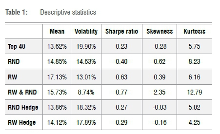
The tactical asset allocation strategy involving the real-world skewness yielded the highest mean return over the sample period with a low variation in returns. The strategy involving the combination of the real-world and risk-neutral moments yielded the lowest variation in returns with a high expected return over our sample period. Low variation in returns, in conjunction with high expected returns, is obviously a desirable property for investment managers.
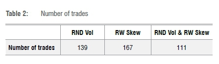
In Table 2, we show the number of trades carried out in each tactical asset allocation strategy shown in Table 1 over the total of 259 forecast months (or 21.5 years).
In the next section, we examine safe withdrawal rates in a forward-looking environment using the tactical asset allocation framework.
Results
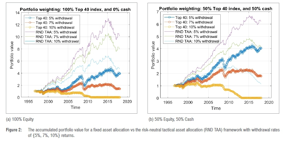
In this section, we assume that a person retired on 1 August 1996 with one unit in retirement savings. The retiree needs to decide how much to withdraw from the retirement fund; draw too much and carry the risk of running out of money, or draw too little and carry the risk of a compromised living standard. Therefore, in this section, we study the life expectancy of a basic retirement portfolio with three commonly used withdrawal rates used in the literature, namely 5%, 7%, and 10% per year of the initial portfolio size. Furthermore, these withdrawals will be adjusted monthly according to inflation rates and historical cash returns - which have been sourced form Firer and McLeod36, Firer and Staunton37, and I-Net - are used in the portfolio.
Safe withdrawal rates
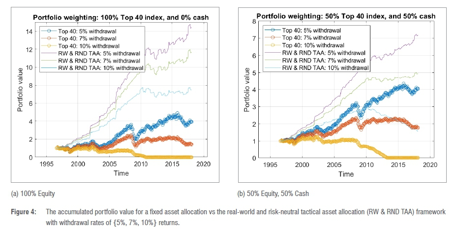
In Figures 2, 3, and 4, we clearly see that the tactical asset allocation framework using the moments obtained from the forward-looking distributions outperformed the fixed asset allocation for the duration of the period under study. Figure 2 shows the accumulated portfolio value for two different asset allocations (see Figures 2a and 2b), with the risk-neutral volatility used in the tactical asset allocation framework described in the section above. Similarly, Figures 3 and 4 show the accumulated portfolio values using the real-world skewness and the combination of the real-world skewness and risk-neutral volatility in the tactical asset allocation framework, respectively. Combining the signal from the risk-neutral volatility and the real-world skewness yielded superior fund prospects for higher withdrawal rates (Figure 4). Although this strategy does not yield the highest mean return over the sample period (Table 1), it has the least variation in returns. Scott et al.6 and Waring and Siegel7 criticised the notion of withdrawing a fixed real amount from an inherently volatile portfolio. This is known as sequence risk. Therefore, reducing the variation in returns is vitally important in determining safe retirement withdrawal rates. This is particularly evident in Figure 4, where a high withdrawal rate of 10% yielded higher portfolio prospects than using only the real-world skewness.
Next, we assess the robustness of the tactical asset allocation framework in determining safe retirement withdrawal rates. In particular, the robust analysis is carried out to determine how much, if any, of the improvement above the commonly quoted 4% safe withdrawal rate is attributed to using forward-looking information, rather than the different market or time periods used in this study.
Robust analysis
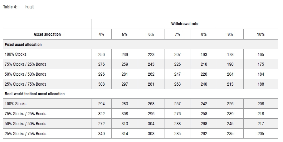
To assess the robustness of the forward-looking distributions in modelling safe withdrawal rates, we carried out a random sampling study. We randomly selected, with replacement, a month from the sample period and used the equity, bonds, and cash returns to generate a one-month sample path. In the tactical asset allocation framework, we also used the previous month's forecasted moments of the randomly selected month to determine the portfolio asset allocation. We then continued to randomly sample from the period to simulate a 30-year period. We, therefore, simulated the evolution of the portfolio over a 30-year period and constructed 10 000 such sample paths. This approach maintains the correlation structure between the assets, as we are using the true observed returns for the selected month for all assets. In Table 3, we show the success rates based on the fixed asset allocation versus the tactical asset allocation framework using the real-world skewness. We found similar results in our sample to the commonly quoted 4% safe withdrawal rate using historical (backward-looking) returns. However, by using forward-looking information in a tactical asset allocation framework, we were able to show significantly improved safe withdrawal rates. Table 4 shows the fugit of the retirement portfolio. In this study, the fugit is defined as the expected duration of the portfolio given that the portfolio fails before the predefined 30-year duration.
It is evident from Table 3 and Table 4 that the simple tactical asset allocation framework, using the forward-looking real-world skewness, yielded superior success and fugit rates to the strategy that involved the fixed asset allocation. As the tactical asset allocation is based on either holding, or selling, the growth asset for a one-month period, the strategy is most prominent with a large growth asset allocation. These results illustrate that one can possibly achieve high portfolio success rates when making use of forward-looking information in portfolio management.
Conclusion
In this study, we used forward-looking information, extracted from observed market-quoted derivative prices, to determine safe retirement withdrawal rates. In particular, we extracted the forward-looking risk-neutral and real-world return distribution functions, and used the distribution moments as a signal in a simple tactical asset allocation framework. We found that using forward-looking information in a tactical asset allocation framework yielded higher portfolio returns with a lower variation in returns compared to the portfolio with a fixed asset allocation.
Many large financial firms frequently extract forward-looking information from derivative securities to infer market sentiment. Therefore, using a forward-looking modelling approach provided a more market consistent analysis of safe retirement withdrawal rates. We found that the portfolio based on the forward-looking real-world skewness in a tactical asset allocation framework supported safe withdrawal rates of up to 7% per annum (inflation adjusted). This strategy obtained similar success rates to the previously quoted 4% safe withdrawal rate determined from the fixed asset allocation based on historical returns. Thus, the performance of the real-world moments, used as a signal in a tactical asset allocation, allows for the possibility of higher withdrawal rates with high success rates. This confirms the usefulness of using forward-looking real-world moments in the management of retirement portfolios to improve the modelling of safe retirement withdrawal rates.
Competing interests
We have no competing interests to declare.
Authors' contributions
V.v.A.: Conceptualisation, methodology, data analysis, writing - the initial draft. E.M.: Conceptualisation, writing - the initial draft, student supervision, project leadership.
References
1. Cooley P Hubbard C, Walz D. Retirement savings: Choosing a withdrawal rate that is sustainable. Journal of the American Association of Individual Investors. 1998;10(1):40-50. [ Links ]
2. Cooley P Hubbard C, Walz D. Sustainable withdrawal rates from your retirement portfolio. Financ Counsel Plan. 1999;20(2):16-21. [ Links ]
3. Bengen W. Determining withdrawal rates using historical data. J Financ Plan. 1994;7(1):171-180. [ Links ]
4. Maré E. Safe spending rates for South African retirees. S Afr J Sci. 2016;112(1/2), Art. #a0138. https://doi.org/10.17159/sajs.2016/a0138 [ Links ]
5. Van Appel V Maré E, Van Niekerk AJ. Quantitative guidelines for retiring (more safely) in South Africa. S Afr Actuar J. 2021;21(1), Art. #4. https://hdl.handle.net/10520/ejc-actu_v21_n1_a4 [ Links ]
6. Scott J, Sharpe W, Watson J. The 4% rule - at what price? J Invest Manag. 2009;7(3):31-48. [ Links ]
7. Waring MB, Siegel LB. The only spending rule article you will ever need. Financial Anal J. 2015;71(1):91-107. https://doi.org/10.2469/faj.v71.n1.2 [ Links ]
8. World Health Organization (WHO). Global health observatory data repository [webpage on the Internet]. c2020 [cited 2021 Nov 14]. https://apps.who.int/gho/data/view.main.SDG2016LEXv?lang=en [ Links ]
9. Purdy M. The first person to live to 150 has already been born. Innovation Hub. 2015 August 8. Available from: https://www.pri.org/stories/2015-08-08/first-person-live-150-has-already-been-born-it-you [ Links ]
10. Ennart H. Âldrandets gâta [The mystery of aging]. Stockholm: Ordfront; 2012. Swedish. [ Links ]
11. Shimko DC. Bounds of probability. Risk (Concord, NH). 1993;6(4):33-37. [ Links ]
12. De Vincent-Humphreys R, Noss J. Estimating probability distributions of future asset prices: Empirical transformations from option-implied risk-neutral to real-world density functions. Bank of England Working Paper no. 455. SSRN; 2012. https://doi.org/10.2139/ssrn.2093397 [ Links ]
13. Scott MC. Assessing your portfolio allocation from a retiree's point of view. Journal of the American Association of Individual Investors. 1996;May:16-19. [ Links ]
14. Abuizam R. A risk-based model for retirement planning. J Bus Econ Res. 2009;7(6):31-43. https://doi.org/10.19030/jber.v7i6.2304 [ Links ]
15. Audrino F, Huitema R, Ludwig M. An empirical analysis of the Ross recovery theorem. SSRN; 2014. http://dx.doi.org/10.2139/ssrn.2433170 [ Links ]
16. Flint E, Maré E. Estimating option-implied distributions in illiquid markets and implementing the Ross recovery theorem. S Afr Actuar J. 2017;17(1):1-28. https://doi.org/10.4314/saaj.v17i1.1 [ Links ]
17. Van Appel V Maré E. The recovery theorem with application to risk management. S Afr Stat J. 2020;54(1):65-91. https://doi.org/10.37920/sasj.2020.54.1.5 [ Links ]
18. Christoffersen P Jacobs K, Chang BY Forecasting with option-implied information. In: Elliott G, Timmermann A, editors. Handbook of economic forecasting. Elsevier; 2013. p. 581-656. https://doi.org/10.1016/B978-0-444-53683-9.00010-4 [ Links ]
19. Hollstein F, Prokopczuk M, Tharann B, Simen CW. Predicting the equity market with option-implied variables. Eur J Financ. 2019;25(10):937-965. https://doi.org/10.1080/1351847X.2018.1556176 [ Links ]
20. Dillschneider Y Maurer R. Functional Ross recovery: Theoretical results and empirical tests. J Econ Dyn Control. 2019;108, Art. #103750. https://doi.org/10.1016/j.jedc.2019.103750 [ Links ]
21. Breeden DT, Litzenberger RH. Prices of state-contingent claims implicit in option prices. J Bus. 1978;51(4):621-651. Available from: https://www.jstor.org/stable/2352653 [ Links ]
22. Malz AM. A simple and reliable way to compute option-based risk-neutral distributions. Federal Reserve Bank of New York Staff Report 677. SSRN; 2014. https://doi.org/10.2139/ssrn.2449692 [ Links ]
23. Aït-Sahalia Y Lo AW. Nonparametric estimation of state-price densities implicit in financial asset prices. J Financ. 1998;53(2):499-547. https://doi.org/10.1111/0022-1082.215228 [ Links ]
24. Gatheral J. A parsimonious arbitrage-free implied volatility parametrization with application to the valuation of volatility derivatives. Presentation at: Global Derivatives and Risk Management; 2004 May 26; Madrid, Spain. [ Links ]
25. Van Appel V, Maré E. The Ross recovery theorem with a regularised multivariate Markov chain. ORiON. 2018;34(2):133-155. https://doi.org/10.5784/34-2-594 [ Links ]
26. Figlewski S. Estimating the implied risk neutral density for the US market portfolio. In: Bollerslev T, Russell JR, Watson M, editors. Volatility and time series econometrics: Essays in honor of Robert F. Engle. Oxford: Oxford University Press; 2010. p. 323-353. https://doi.org/10.1093/acprofioso/9780199549498.003.0015 [ Links ]
27. Bollerslev T, Tauchen G, Zhou H. Expected stock returns and variance risk premia. Rev Financ Stud. 2009;22(11):4463-4492. https://doi.org/10.1093/rfs/hhp008 [ Links ]
28. Shackleton MB, Taylor SJ, Yu P. A multi-horizon comparison of density forecasts for the S&P 500 using index returns and option prices. J Bank Financ. 2010;34(11):2678-2693. https://doi.org/10.1016/j.jbankfin.2010.05.006 [ Links ]
29. Aït-Sahalia Y, Lo AW. Nonparametric risk management and implied risk aversion. J Econometrics. 2000;94(1-2):9-51. https://doi.org/10.1016/S0304-4076(99)00016-0 [ Links ]
30. Bliss RR, Panigirtzoglou N. Option-implied risk aversion estimates. J Financ. 2004;59(1):407-446. https://doi.org/10.1111/j.1540-6261.2004.00637.x [ Links ]
31. Hansen LP, Renault E. Pricing kernels and stochastic discount factors. In: Cont R, editor. Encyclopedia of quantitative finance. Chichester: John Wiley & Sons; 2010; p. 1418-1427. [ Links ]
32. Ross S. The recovery theorem. J Financ. 2015;70(2):615-648. https://doi.org/10.1111/jofi.12092 [ Links ]
33. Chakraborty S. Generating discrete analogues of continuous probability distributions - A survey of methods and constructions. J Stat Distrib. 2015;2(6):1-30. https://doi.org/10.1186/s40488-015-0028-6 [ Links ]
34. Cuesdeanu H, Jackwerth JC. The pricing kernel puzzle: Survey and outlook. Ann Finance. 2018;14:289-329. https://doi.org/10.1007/s10436-017-0317-9 [ Links ]
35. Thomson D, Van Vuuren G. Forecasting the South African business cycle using Fourier analysis. Int Bus Econ Res J. 2016;15(4):175-192. https://doi.org/10.19030/iber.v15i4.9755 [ Links ]
36. Firer C, McLeod H. Equities, bonds, cash and inflation: Historical performance in South Africa 1925 to 1998. Invest Anal J. 1999;28(50):7-28. https://doi.org/10.1080/10293523.1999.11082398 [ Links ]
37. Firer C, Staunton M. 102 Years of South African financial market history. Invest Anal J. 2002;31(56):57-65. https://doi.org/10.1080/10293523.2002.11082442 [ Links ]
 Correspondence:
Eben Maré
Email: Eben.Mare@up.ac.za
Received: 04 Aug. 2021
Revised: 14 Nov. 2021
Accepted: 30 Nov. 2021
Published: 29 Mar. 2022
EDITOR: Michael Inggs
FUNDING: None

