RESEARCH ARTICLE

 

Impact of heat and moisture stress on crop productivity: Evidence from the Langgewens Research Farm

 

 

Beatrice Conradie^I; Jenifer Piesse^{II, III}; Johann Strauss^IV

^ISchool of Economics, University of Cape Town, Cape Town, South Africa
^IIDepartment of Management, King's College London, London, United Kingdom
^IIIDepartment of Agricultural Economics, Stellenbosch University, Stellenbosch, South Africa
^IVWestern Cape Department of Agriculture, Stellenbosch, South Africa

Correspondence

 

 

---

ABSTRACT

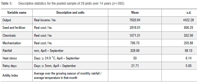
We investigated the effect of heat and moisture stress on total factor productivity in crop farming under experimental farm conditions. Heat stress is the number of days during the growing season during which the maximum temperature exceeds 24.9 °C. Total rainfall is treated as a basic factor of production and periodic moisture stress, or lack thereof, is the number of rainfall days during the growing season. All models controlled for the cumulative soil benefits arising from minimum tillage, which is the main objective of the experiment. Model specification was evaluated using likelihood ratio tests and three are worthy of note. The study site received 329 mm of rainfall on average on 22 rainy days per season during the period 2002-2015, while the maximum temperature typically rose above 24.9 °C on 33 days per growing season. The average efficiency of the plots in the long-term crop rotation experiment increased at 3.4% per year from a base of 60% to the most recent level of 78%. Neither heat nor moisture stress changed significantly over the study period. Heat stress was found to reduce efficiency by 1.75% per hot day and rainfall increased efficiency by 1.45% for each additional rainy day. However, the interaction of heat and moisture stress lowered productivity overall.
SIGNIFICANCE:
• This study contributes a new approach to modelling the effect of climate on agricultural productivity using a new metric of heat and moisture stress.
• We quantify the marginal effects of rising temperatures and rainfall events and evaluate several potential specifications of heat and moisture stress variables.

Keywords: total factor productivity, climate, rainfed arable farming, experimental farm environment, Langgewens Research Farm

---

 

 

Introduction

A global rise in temperature is a feature of climate change and is likely to impact rainfall, both in the level and in the distribution. However, there remains some uncertainty about the heat and moisture stress relationship between these environmental phenomena. It is predicted that 20% lower rainfall combined with a 2 °C increase in temperature would reduce profitability in field crops in South Africa by 4.4%.¹ That is, if the temperature rose by 3 °C, profits would fall by 11.7%, although should this increase be accompanied by moderate rainfall, real profits may increase. The prediction for the Northern and Western Cape Provinces of South Africa is a 1.5-2 °C rise in surface temperatures combined with a 5-10% lower median rainfall by the turn of the century.² Thus, if the predictions are right, there is no real threat overall from climate change, except for wheat production in the winter rainfall area, which will be stressed by rising temperatures.

However, given the absence of any certainty with respect to long-term meteorological forecasts, we investigated the effects of current rainfall and temperature ranges on the performance of dryland wheat production in the Western Cape. Clearly, the more precisely the climate variables can be measured, the more valuable the efficiency of producers facing these environmental factors is to policymakers and practitioners alike. Our approach was based on Ricardian climate models, although here there is a different dependent variable from those used earlier, as well as an emphasis on capturing climate stress. In the Mendelsohn et al.³ analysis, land prices were used as a proxy for expectations about future income. By explaining land prices with average rainfall and temperature, cross-section variation can be used to predict how changing climate is likely to affect the global food system, given controls for soil potential etc. Due to the lack of suitable farm sales data, the World Bank abandoned land prices as a dependent variable in their studies in favour of net farm income or yield⁴, and this approach is replicated here. Sales and net farm income are closely correlated, with expected net revenue per hectare obtained from data on farm sales prices by assuming a suitable discount rate, whereas yield is equivalent to net revenue at fixed prices. In both cases it is important to assume a given level of technical progress and expectations about how climate change will present in the future. If either yield or net revenue replaces land prices, the model loses much of its original elegance, as these additional factors now have to be controlled for explicitly.

 

Review of the literature and contribution of this paper

Ricardian models are frequently used to analyse agricultural production and are derived from the simple observation that the value of land reflects its net productivity. Most authors use a cross-sectional approach. A major influence on this paper was Mendelsohn et al.'s³ study in which controls were included to account for eight soil characteristics, along with altitude, latitude (as a proxy for solar radiation), per capita income and population density, the latter to take account of opportunities in the non-farm sector. Yield was modelled as a quadratic function of rainfall and temperature whilst seasonal rainfall and temperature effects were included as separate variables. Gbetibouo and Hassan¹ build on Mendelsohn et al.³ by using the Ricardian model to capture the effect of rainfall and temperature variability on land productivity and land values, although they only considered long-term spatial variation and ignored temporal variability between and within seasons. Kurukulasuriya et al.⁵ modelled net farm income per hectare in several African countries, using access to electricity as a proxy for modern infrastructure, while Gbetibouo and Hassan¹ introduced the size of the farm labour force in addition to population density to capture potential macroeconomic shifts.

The Ricardian approach has continued to evolve, such as moving to more interesting dimensions and transformations of the data, including panel data⁶ and first differences in a time series model⁷. Cabas et al.⁸ summarised many of the site characteristics in an area change variable based on the supposition that yields will fall and become more erratic when production expands onto marginal land. The same analysis included technical change and input price variation and introduced climate volatility using the mean of the coefficient of variation (the standard deviation divided by the mean) of both rainfall and temperature. Temperature is the mean daily value while rainfall is in total millimetres recorded during the growing season. Following the principles of phenology, the growing season begins when temperatures rise above 5 °C for five consecutive days and is computed from monthly average data. In Boubacar⁹, the yield response model was reduced to two moisture stress variables, beneficial temperature was measured in growing degree days, technical progress and a somewhat dubious area change variable accounted for unexplained dynamics. The first moisture stress variable captured drought periods as a percentage of expected rainfall while the second identified the month with the highest share of annual rainfall to capture variability.

The literature on Ricardian modelling is clear about how to capture climate fixed effects; yield is usually specified as a quadratic function of total rainfall and mean temperature. Dinar et al.¹⁰ went a step further by defining an aridity index as mean temperature divided by mean rainfall, which formed part of the frontier sub-model. Roux¹¹ expressed a similar idea by defining a relative drought tolerance index as rainfall squared divided by its standard deviation, although this index was never used in productivity modelling. With respect to estimation, it became important to consider seasonal differences as Ricardian models began to be estimated with panel data. Cabas et al.⁸ captured variability as a fixed effect with the coefficient of variation of rainfall, temperature and growing degree days, although this method still does not reflect the difference in variability between one season and the next. Employing adverse climate as an explanation for the observed differences in farm-level efficiency requires a specification that captures climate stress, which is site specific. In the northern latitudes of Canada, temperature stress comes in the form of low temperatures, best measured as growing degree days⁸, although this does not limit wheat growth in South Africa while heat stress does.¹²

This paper contributes to the literature in two ways. Firstly, there is currently no credible model that considers comprehensive weather changes in productivity. Therefore, we used time series data from a multiplot crop rotation experiment at a single research site and focussed on measuring year-on-year differences in the amount of heat and moisture stress. Secondly, we used a novel approach to estimation, by extending the standard stochastic frontier production function with inefficiency effects.¹³ In this model, a best-practice frontier was jointly estimated with an inefficiency model that explains individual performance relative to the benchmark. Inputs and outputs into the production process were considered and the typical explanations for inefficiency in this well-rehearsed literature usually include some combination of technology, subsidies, governance and extension factors. Resource quality, such as access to irrigation, has formed part of the explanation right from the start and can appear as part of the frontier or in the inefficiency model.^13,14 Finally, by adding enhanced proxies for moisture and heat stress, the standard model was adapted for monitoring climate change impacts on agricultural productivity.

 

Methods and data

The established dependent variable in the Ricardian model is yield, or profitability, where the latter is yield at current prices for a given technology. Alternatively, land values can be used, which is the present value of the expected future income stream at constant prices. We propose that a total factor productivity score replace yield as the dependent variable. This measure has the advantage of being independent of prices and capable of capturing both technical change and changing factors of production.

The stochastic frontier production function model with climate-based inefficiency effects uses input and output data to fit a benchmark (Equation 1) and various proxies for temperature and rainfall limitations to production to explain deviations from the benchmark (Equation 2). Instead of referring to farms, as is usually done, the inefficiency scores predicted by this two-part model refer to experimental plots of a quarter hectare each. These plots form part of one of four crop rotation systems that are being compared to other crop-livestock rotation systems at Langgewens Research Farm in the Western Cape, South Africa (33°17'0.78"S, 18°42'28.09"E). The data were provided by the researchers at the farm and we checked the information using standard robustness tests. The site's average annual rainfall since 1964 is 403 mm and almost 80% of it falls during the winter growing season, from April to September.

The productivity model can be stated as:

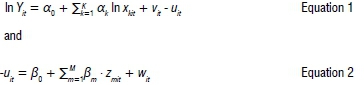
where Y is output, x is input, z potential explanations for deviations from the frontier (inefficiency effects), and a and ß are parameters to be estimated. The error term w_it in Equation 2 is a typical normally distributed error term. In Equation 1, the error term is decomposed into a normally distributed component, v_it, and a one-sided inefficiency term, u_it, which captures each observation's degree of deviation from the benchmark. Output is measured as the natural logarithm of the real value of product sales and nominal values were deflated using the general consumer price index published in the Abstract of Agricultural Statistics.¹⁵ The rotations incorporated here are a wheat monoculture, a wheat-canola rotation and two systems that rotate wheat and canola with lupins. Two thirds of the observations are for wheat, while 21% apply to canola and 14% to lupins. The data are from one crop rotation trial at the research facility. Decisions like fertiliser applications and planting dates are jointly controlled by the responsible researcher and farm manager. Inputs are bought on tender and output is sold on the open market. The inputs are seed and fertiliser cost, chemicals (pesticides herbicides and fungicides), mechanisation cost and total seasonal rainfall. Rainfall is measured in millimetres recorded during the growing season (April -September). The inputs in value terms are in constant 2010 ZAR prices deflated according to the input specific deflators in the Abstract and logged. As in all well-behaved production functions, a is expected to be positive and significant.

Pooled descriptive statistics for the study period, 2002-2015, are shown in Table 1. Land is obsolete as plot data are expressed per hectare, and, because labour is used in fixed proportion to machinery, it is omitted to avoid collinearity.

Instead of modelling crop performance as a function of mean rainfall and temperature as Ricardian models do, we specifically wanted to capture heat and moisture stress on the total factor productivity of each crop in the production system. The simplest formulation for heat stress is a count of growing days on which the maximum temperature reaches an arbitrary threshold. After experimenting with several, we opted for 24.9 °C which is often used for wheat.¹² While output is correlated with total rainfall, total rainfall does not capture the effect of periodic moisture stress. The standard deviation of rainfall, or its coefficient of variation, has been used as a measure of variability.⁸ Given the construction of this statistic, the higher the standard deviation for a given level of rainfall, the higher its coefficient of variation. With total rainfall already in the stochastic frontier, it was logical to use the standard deviation of rainfall in the inefficiency model. This was calculated from daily observations over the growing season (April - September) and predicted a higher standard deviation to cause more inefficiency. The product of the two, which would capture the interaction of temperature and moisture stress, was predicted to increase inefficiency.

A number of specifications were estimated. Dinar et al.¹⁰ combined temperature and heat effects into an aridity index, defined as the ratio of annual mean daily temperature over total annual rainfall. This variable was tested independently and in combination with the seasonal heat and moisture stress variables described above. The aridity index is for the growing season only. Mean daily temperature was calculated by taking the average of the daily minimum and maximum and then the average over the growing season to compute the average mean daily temperature for the growing season. This was divided by total rainfall recorded during the growing season. The prediction was that greater aridity would increase inefficiency.

In another specification, the standard deviation of rainfall as a proxy for moisture stress was replaced by a count of rainy days, defined as 24-h periods that receive more than 5 mm of rainfall. For a given total seasonal rainfall an increase in the number of rainy days implies shorter periodic droughts, which ought to decrease inefficiency. Generalised likelihood ratio tests were used to choose between nested specifications, but this test does not allow the choice between the different ways of capturing periodic drought. There we were guided by the overall goodness of fit and the signs and significance of the input elasticities.

This study took place against the backdrop of soil improvements after the adoption of zero tillage, which is expected to raise productivity. Langgewens Research Farm switched to minimum tillage in 1996 and adopted zero tillage in 2002. Dramatic improvements in soil conditions followed and this is captured in Equation 2 by a time trend, which is the usual method of accounting for technical change. Winter rains failed in 2003 (67% of expected seasonal rainfall), 2004 (62%) and 2015 (54%), and 2007 was an exceptionally good year (141% of expected seasonal rainfall). In 2003, most plots performed sufficiently well to be harvested. By 2015, the same plots did well under similar conditions. The soil gains include higher carbon levels that improve soil structure, permeability and fertility, and on some plots rotating monocotyledon with dicotyledon crops lowers weed pressures enough to cut down on herbicide inputs.¹²

As no new varieties or production methods featured in the experiment during the study period and given the low technical progress in dryland crop farming on commercial farms in the Western Cape during the second half of the 20th century¹⁶, it was unlikely that the system would also experience Hicks-neutral technical progress and so there was no need to include a time trend in the frontier model.

Equation 4 gives the Battese and Corra¹⁷ parameterisation of the inefficiency term, in which gamma is calculated as follows:

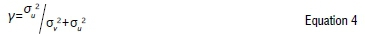
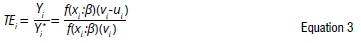
The efficiency scores predicted by Equation 3 vary from zero to one, or 0-100%. Observations close to 100% set the benchmark, but as the model allows for statistical noise, the best performing plots are usually no more than 97% efficient under optimal conditions, although mean scores vary with model complexity and sample size. For experimental plot data, where mismeasurement is negligible, gamma could approach unity.

The translog functional form has become standard in total factor productivity estimates, and is often accompanied by a log-likelihood test that compares its performance to that of Cobb Douglas. The benefit of estimating a more general functional form is that it relaxes the assumption of constant elasticities of substitution made by Cobb Douglas. However, in this case, in which there is a single manager in control of day-to-day production decisions for all plots on the experimental farm, the Cobb Douglas was considered sufficient, especially as it allows more degrees of freedom to experiment with climate variables.

 

Results and discussion

This section is divided into four parts. The first part presents the baseline model, which has only the cumulative no tillage benefits and heat stress in the inefficiency equation. The second part introduces periodic drought stress in the form of a standard deviation on seasonal rainfall as a third z-variable. The number of rainy days replaces the standard deviation of rainfall in the third part and the performance of the Dinar aridity index is evaluated in the fourth part. The same procedure was followed with all three proxies and all results in the tables first present the frontier specification and then the results of the inefficiency model. Once the suitability of the basic proxy had been confirmed, it was interacted with the heat stress variable to determine if there was a joint effect.

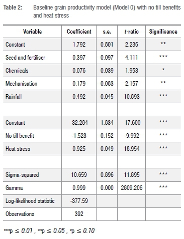
The baseline model with no tillage benefits and heat stress

The baseline specification works well here. All four Cobb Douglas input coefficients have the expected sign and are significant at p < 0.10. The output elasticities indicate that output is most closely correlated to total seasonal rainfall, where a 1% increase in rainfall will result in a 0.49% increase in the real value of output. The second largest output elasticity is on seed and fertiliser, where a 1% increase in expenditure is predicted to result in a 0.40% increase in output. This is followed by mechanisation whose output elasticity is 0.179 and agro-chemicals whose output elasticity is 0.076. The relative unimportance of agro-chemicals in this production system explains why its coefficient is measured with such a relatively low level of certainty.

The inefficiency model performs equally well. By relaxing the mean response function assumption of independently and identically distributed error terms, the stochastic frontier model presented in Table 2 is estimated with four additional parameters - sigma-squared, gamma, the no tillage benefit and the heat stress coefficient, all of which are significantly different from zero. The log-likelihood value of the mean response function was -752.99, while the stochastic frontier model yielded a value of -377.59. A likelihood ratio test was performed to test that the four restrictions were valid. The test statistic of LR = -2(-752.99 - (-377.99)) = 750.80 rejects the mean response model at the highest level of significance. The critical value is 12.483 for p < 0.01 . It is clear from these tests that the stochastic frontier function form fits the data better than the ordinary least squares estimation. The mean efficiency of the pooled sample is 55%, the cumulative benefit of the practice of zero tillage is 3.45% per year and an extra day of heat stress during the growing season reduces efficiency by 1.78% across all crops and rotations in the sample.

 

 

Is the coefficient of variation of rainfall a valid proxy for periodic moisture stress?

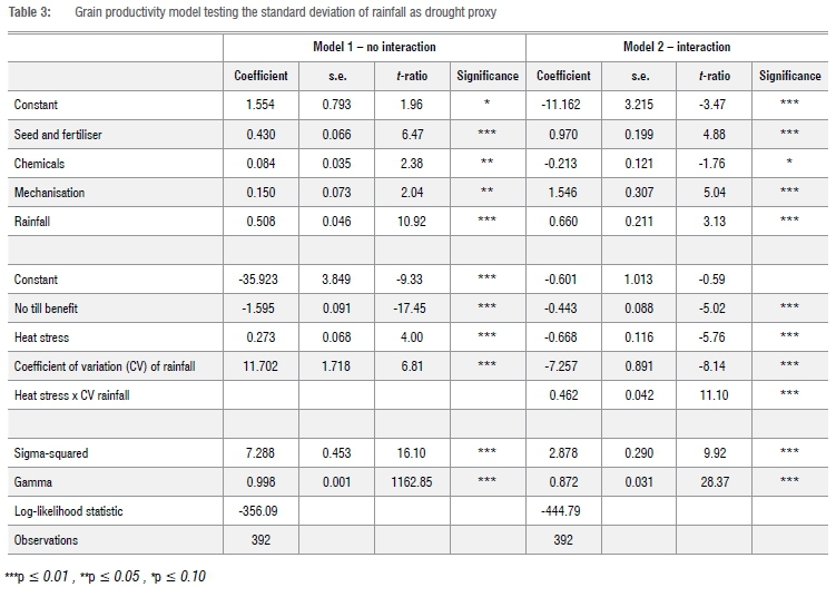
Introducing the coefficient of variation of seasonal rainfall into the inefficiency sub-model produced a plausible stochastic frontier production function and confirmed the expectations about the effects of zero tillage and heat stress on plot-level efficiency. The output elasticities are all significant and have similar magnitudes as before. The no tillage benefit increases fractionally to 3.54% per year. The negative impact associated with an additional day of heat stress goes up to 1.79%. The restrictions imposed by the mean response function are rejected with a log-likelihood test statistic of 793.79, and when compared to the result in Table 2, the hypothesis that the standard deviation of rainfall is unrelated to plot-level efficiency is rejected with a test statistic of LR = -2(-377.59 - (-356.09)) = 43.00. The regression coefficient on the coefficient of variation of rainfall is positive and significant, confirming it as a reasonable proxy for rainfall variability. A 1% increase in variability increases inefficiency by 0.36%.

The productivity frontier is less robust when the number days of heat stress is interacted with the coefficient of variation of seasonal rainfall (see Table 3). The relative sizes of the input elasticities in the production function sub-model change dramatically compared to the baseline and Model 1. The sign on the coefficient on chemicals becomes negative and heat stress changes from a stress factor to an enhancer of productivity. Another reason for rejecting this specification is that, in this model, the log-likelihood statistic is much lower than that of Model 1.

The analysis was repeated with the standard deviation of rainfall instead of the coefficient of variation, with much the same result. These are not shown. In the equivalent of Model 1, two important coefficients were no longer significantly different from zero, namely chemicals and the drought proxy, but all signs were as expected. The log-likelihood statistic was lower than in Model 1. Interacting heat stress with the standard deviation of rainfall caused fewer problems than it did in Model 2. In the equivalent of Model 2, the coefficient on chemicals was insignificant, although its sign remained positive. The coefficient on heat stress remained positive although the sign on the standard deviation of rainfall became negative and the sign on the interaction term was positive. The log-likelihood statistic was -383.42, an improvement on Model 2, but the interpretation on the coefficient of the interaction term is less straightforward than it had been in Model 2. Therefore, neither coefficient of variation on rainfall nor the standard deviation of rainfall worked particularly well as proxies for periodic drought.

Can rainy days capture periodic droughts or the lack thereof?

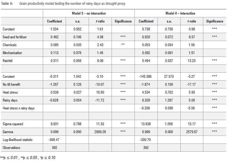
Conceptually, rainy days are an enhancer rather than a stressor of crop productivity and the simple count format is easy to interpret. Replacing the coefficient of variation with this count variable produced the results in Table 4. Model 3, the specification with no interaction term between heat stress and rainfall effects, performed almost as well as Model 1. The input elasticities were similar, the inefficiency sub-model's results were as expected and the only difference was that the coefficient on mechanisation was not significantly different in Model 3. Mean efficiency was 56% and the scores increased by 3.43% per year due to the benefits of zero tillage. The magnitude of the heat stress penalty of 1.75% per additional day above 24.9 °C was similar to that in Model 2. That is, each rainy day increases productivity by 1.45%. Because the positive effect of a rainy day was smaller than the negative effect of a heat stress day, the interaction term was expected to carry the same sign as heat stress.

A likelihood ratio test was used to determine if the coefficient on the interaction term in Model 4 should be included. The result was that the coefficient is not zero. The test statistic of Model 3 as a restriction of Model 4 yielded a test statistic of LR = 75.47. This is an anomaly as neither chemicals nor mechanisation produced significant coefficients in Model 4. There were other problems in the inefficiency model too. All four coefficients were significant and the no tillage benefit and heat stress produced the expected signs, but rainy days became a stressor while the combined effect of heat stress and rainy days was positive. While the latter could mean that temperatures above 25 °C are not a problem if there is enough moisture in the soil profile, it is inconceivable that more frequent rainfall on its own would have a negative impact on productivity.

Does an aridity index simplify matters?

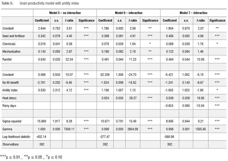
The aridity index used in the results in Table 5 was adapted from Dinar et al.¹⁰ In Model 5, the simplest specification, where the aridity index is combined only with the cumulative no tillage benefit, the coefficient on the former is positive and significant. This result is consistent with the result produced by Model 3 in Table 4 because the aridity index rises with heat stress and falls with more frequent precipitation. The differences between the two models are minor. In Model 3 heat stress is defined according to an arbitrary cut-off, while in Model 5 there is no temperature cut-off assumed. With respect to rainfall, Model 5 does not consider the distribution of rainfall, which Model 3 does. In both cases, only three of the four input elasticities are significantly different from zero, but the variables that are not significant are different between the models, including the elasticity on chemicals which is much lower than previously found.

In Model 6 the heat stress count variable was added. This specification is most like the baseline model in Table 2 because it does not include any rainfall proxy other than total rainfall in the production frontier. Including the heat stress count variable makes the aridity index insignificant, although a likelihood ratio test rejects its exclusion. The test value is LR = 109.34. This time all the elasticities are plausible and significant at p < 0.10, while the coefficient on the aridity index, although still positive, is no longer statistically significant.

The final specification in Model 7 added the number of rainy days recorded during the rainy season, which improved the fit slightly compared to Model 6. The frontier performs well, despite the smaller elasticity on mechanisation and its lack of significance. The results of the inefficiency model are better than all the earlier specifications. More time after the adoption of zero tillage significantly decreases inefficiency, more heat stress increases inefficiency and more rainy days decreases inefficiency. All of this is the same as in Model 3 in Table 4. However, in Model 7, the aridity index provides an interaction effect between rainfall and temperature. The coefficient is significant at p < 0.10 and negative, which means that inefficiency is negatively correlated with aridity. However, interpreted as an interaction term of rainfall and temperature, the negative sign could mean that the net effect is determined by rainfall and not by heat stress. The low level of significance suggests that the net effect is site specific, which seems eminently reasonable. The mean efficiency and the percentage change in efficiency scores per year of zero tillage, or heat stress or rainy day recorded during the growing season, are stable across specifications.

 

Conclusions

We used experimental farm data to investigate the impact of climate change on productivity in South Africa, importantly using a new approach for rainfall and temperature stress. The approach followed the Ricardian models used in the literature but extended these in two important respects. Firstly, the data are for a single location, although many different plots were included and the analysis was able to capture changes over time. Secondly, the standard Ricardian specification was estimated using a stochastic frontier with inefficiency effects, which made it possible to allocate the results to the plot level.

The many specifications in which proxies for heat and moisture stress have been used to explain crop plot efficiency and the result provide confidence that this approach is viable and can be extended to encompass other environments and other contexts. The main implications of the results are twofold. Firstly, climate change will have consequences for farm efficiency, and secondly, something can be done about it. This first conclusion is already visible in how plot level efficiencies respond to the temperature and rainfall variation documented at the site over the last decade and a half, regardless of whether this variation is considered normal or a sign of permanent climate change. If either rainfall or temperature is likely to become more variable in future, farm productivity will decrease as a result, and not just become more variable as previously suggested.¹⁸

The positive results of this research show that, while little can be done to influence rainfall or temperature, at least in the short term, producers can choose their production system. In the Langgewens experiment, the first 14 years of zero tillage production practices resulted in an almost 3.5% increase in productivity every year, across good and bad seasons. This effect is unlikely to be linear, and so the marginal efficiency benefits will probably decline as soil benefits mature, and finding the shape and length of the lag structure involved is a topic for further research. Certainly, it is not known at this stage how long the benefits take to mature and there is a difference in the rate at which the benefits accumulate across different rotation systems. Finally, from a modelling point of view, efficiency can replace crop yield or its derivatives in climate models, and the Dinar aridity index is worth pursuing; capturing rainfall variability with a coefficient of variation does not work quite as well as a simple count variable. All of these preliminary conclusions can be usefully re-examined in other contexts. What is without doubt is that careful collection of climate data along with production variables is essential.

 

Acknowledgements

We acknowledge the input of the two anonymous reviewers.

 

Competing interests

We have no competing interests to declare.

 

Authors' contributions

B.C.: Conceptualisation, data cleaning, empirical analysis, first draft. J.P: Conceptualisation, final draft. J.S.: Data collection.

 

Data availability

Data are available on request from Johann Strauss (JohannSt@elsenburg.com) and subject to permission from the Western Cape Department of Agriculture.

 

References

1. Gbetibouo GA, Hassan RM. Measuring the economic impact of climate change on major South African field crops: A Ricardian approach. Glob Planet Change. 2005;47(2-4):143-152. https://doi.org/10.1016/j.gloplacha.2004.10.009        [ Links ]

2. Water Research Commission, South African Weather Service. A climate change reference atlas based on CMIP5-CORDEX downscaling [document on the Internet]. c2017 [cited 2019 Aug 12]. Available from: http://www.weathersa.co.za/Documents/Climate/SAWS_CC_REFERENCE_ATLAS_PAGES.pdf        [ Links ]

3. Mendelsohn R, Nordhaus WD, Shaw D. The impact of global warming on agriculture: A Ricardian analysis. Am Econ Rev. 1994:753-771.         [ Links ]

4. Sanghi A, Mendelsohn R, Dinar A. The climate sensitivity of Indian agriculture. In: Dinar A, Mendelsohn R, Evenson R, Parikh J, Sanghi A, Kumar K, et al. (eds). Measuring the impact of climate change on Indian agriculture. World Bank Technical Paper number 402. Washington DC: World Bank; 1998. p. 69-139.         [ Links ]

5. Kurukulasuriya P, Mendelsohn R, Hassan R, Benhin J, Deressa T, Diop M, et al. Will African agriculture survive climate change? World Bank Econ Rev. 2006;20(3):367-388. https://doi.org/10.1093/wber/lhl004        [ Links ]

6. Massetti E, Mendelsohn R. Estimating Ricardian models with panel data. Clim Chang Econ. 2011;2(04):301-319. https://doi.org/10.1142/s2010007811000322        [ Links ]

7. Mwaura FM, Okoboi G. Climate variability and crop production in Uganda. J Sustain Dev. 2014;7(2):159. https://doi.org/10.5539/jsd.v7n2p159        [ Links ]

8. Cabas J, Weersink A, Olale E. Crop yield response to economic, site and climatic variables. Clim Change. 2010;101(3-4):599-616. https://doi.org/10.1007/s10584-009-9754-4        [ Links ]

9. Boubacar I. The effects of drought on crop yields and yield variability: An economic assessment. Int J Econ Finance. 2012;4(12):51-60. https://doi.org/10.5539/ijef.v4n12p51        [ Links ]

10. Dinar A, Karagiannis G, Tzouvelekas V. Evaluating the impact of agricultural extension on farms' performance in Crete: a nonneutral stochastic frontier approach. Agricultural Economics. 2007 Mar;36(2):135-46. https://doi.org/10.1111/j.1574-0862.2007.00193.x        [ Links ]

11. Roux PW. South Africa devises scheme to evaluate drought intensity. Drought Network News. 1991;3(3):18-23.         [ Links ]

12. MacLaren C, Storkey J, Strauss J, Swanepoel P Dehnen-Schmutz K. Livestock in diverse cropping systems improve weed management and sustain yields whilst reducing inputs. J Appl Ecol. 2019;56(1):144-156. https://doi.org/10.1111/1365-2664.13239        [ Links ]

13. Battese GE, Coelli TJ. A model for technical inefficiency effects in a stochastic frontier production function for panel data. Empir Econ. 1995;20(2):325-332. https://doi.org/10.1007/bf01205442        [ Links ]

14. Piesse J, Conradie B, Thirtle C, Vink N. Efficiency in wine grape production: Comparing long-established and newly developed regions of South Africa. Agric Econ. 2018;49(2):203-212. https://doi.org/10.1111/agec.12409        [ Links ]

15. South African Department of Agriculture Fisheries and Forestry (DAFF). Abstract of agricultural statistics. Pretoria: DAFF; 2018.         [ Links ]

16. Conradie B, Piesse J, Thirtle C. District-level total factor productivity in agriculture: Western Cape Province, South Africa, 1952-2002. Agric Econ. 2009;40(3):265-280. https://doi.org/10.1111/j.1574-0862.2009.00381.x        [ Links ]

17. Battese GE, Corra GS. Estimation of a production frontier model: with application to the pastoral zone of Eastern Australia. Aust J Agric Econ. 1977;21(3):169-179. https://doi.org/10.1111/j.1467-8489.1977.tb00204.x        [ Links ]

18. Speranza CI, Kiteme B, Wiesmann U. Droughts and famines: The underlying factors and the causal links among agro-pastoral households in semi-arid Makueni district, Kenya. Glob Environ Change. 2008;18(1):220-233. https://doi.org/10.1016/j.gloenvcha.2007.05.001        [ Links ]

 

 

Correspondence:
Beatrice Conradie
Email: Beatrice.conradie@uct.ac.za

Received: 16 Sep. 2020
Revised: 21 Apr. 2021
Accepted: 04 May 2021
Published: 29 Sep. 2021

 

 

Editors: Teresa Coutinho, Salmina Mokgehle
Funding: None