RESEARCH ARTICLE

 

Model inter-comparison for short-range forecasts over the southern African domain

 

 

Patience T. Mulovhedzi^I; Gift T. Rambuwani^I; Mary-Jane Bopape^I; Robert Maisha^I; Nkwe Monama^{II, III}

^ISouth African Weather Service, Pretoria, South Africa
^IICentre for High Performance Computing (CHPC), Council for Scientific and Industrial Research, Pretoria, South Africa
^IIINational Integrated Cyber-Infrastructure System (NICIS), Council for Scientific and Industrial Research, Pretoria, South Africa

Correspondence

 

 

---

ABSTRACT

Numerical weather prediction (NWP) models have been increasing in skill and their capability to simulate weather systems and provide valuable information at convective scales has improved in recent years. Much effort has been put into developing NWP models across the globe. Representation of physical processes is one of the critical issues in NWP, and it differs from one model to another. We investigated the performance of three regional NWP models used by the South African Weather Service over southern Africa, to identify the model that produces the best deterministic forecasts for the study domain. The three models - Unified Model (UM), Consortium for Small-scale Modelling (COSMO) and Weather Research and Forecasting (WRF) - were run at a horizontal grid spacing of about 4.4 km. Model forecasts for precipitation, 2-m temperature, and wind speed were verified against different observations. Snow was evaluated against reported snow records. Both the temporal and spatial verification of the model forecasts showed that the three models are comparable, with slight variations. Temperature and wind speed forecasts were similar for the three different models. Accumulated precipitation was mostly similar, except where WRF captured small rainfall amounts from a coastal low, while it over-estimated rainfall over the ocean. The UM showed a bubble-like shape towards the tropics, while COSMO cut-off part of the rainfall band that extended from the tropics to the sub-tropics. The COSMO and WRF models simulated a larger spatial coverage of precipitation than UM and snow-report records.
SIGNIFICANCE:
• Extreme weather events, such as tornadoes, floods, strong winds and heat waves, have significant impacts on society, the economy, infrastructure, agriculture and many other sectors. These impacts may be mitigated or even prevented through early warning systems which depend on the use of weather forecasts and information from NWP models. As South Africa depends on models from developed countries, these models may have shortcomings in capturing extreme weather events over the southern African region.

Keywords: numerical weather prediction models, convective scale, physical process, model inter-comparison, South African Weather Service

---

 

 

Introduction

Weather and climate impact everyday life, while extreme events can cause loss of life and injuries as well as damage to property. The impacts of adverse weather events can be reduced if effective early warnings exist. Numerical weather prediction (NWP) is an integral part of early weather warnings because it provides weather forecasters with a longer lead time than what is available in the now-casting timescale. NWP models are based on the laws of physics that govern atmospheric dynamics and thermodynamics, and they use observations as inputs to forecast the future state of the atmosphere.^1-3 This process has improved significantly over recent years due to several factors. These factors include an improved understanding and representation of physical and dynamical processes in models, advances in observation technology and data assimilation techniques, and improved computational resources and capabilities^2-4 that make it possible for NWP models to run at high resolutions like a few kilometres to hundreds of metres. The advantage of running such NWP models include improved model forecast skill such as accurate numerical prediction of near-surface weather conditions (e.g. clouds, fog, frontal precipitation) and simulation of severe weather events triggered by deep moist convection (supercell thunderstorms, intense mesoscale convective complexes, prefrontal squall line storms, tornadoes and heavy snowfall from wintertime mid-latitude cyclones)^5,6 as well as heatwaves⁷. In addition, NWP models allow for formation of structures recognisable as convective clouds and can simulate cloud microphysics such that updraught life cycle and downdraught generation are addressed fairly.¹

Depending on several factors - such as the design of a forecasting system, model configuration, initial conditions for the model, and lateral and surface boundary conditions - different NWP models produce variable forecasts across different parts of the globe.^1,6,8 Southern Africa is characterised by numerous climatic regions that range from arid to temperate and Mediterranean winter-rainfall regions.^9-11 These regions are affected by different weather systems during different seasons, and have variable characteristics. In addition, the southern hemisphere has a higher sea area compared to land cover, which also has an effect on weather systems.¹² As a result, the simulation of these systems requires specific model parameterisation configurations which are compatible with the region, and which take into account localised influences such as land cover, soil moisture, and cloud processes.^13,14 The weather systems may vary in horizontal scale, duration, and intensity, resulting in different effects on communities. Therefore, it is critical to identify a highly skilled NWP model that can capture the weather events that affect the study domain.

Representation of physical (sub-grid) processes differs in NWP models, such that different inter-comparison studies have been developed.^8,15-17 Dabernig et al.⁸ conducted a model inter-comparison study to identify the most suitable model for predicting wind power over parts of Europe. Four NWP models or configurations were used: global deterministic European Centre for Medium-Range Weather Forecasts (ECMWF-DET), regional deterministic of the Austrian weather service (ALARO), ECMWF global ensemble prediction system (ECMWF EPS), and ECMWF global ensemble hindcast and reforecast of global ensembles (ECMWF-HC and GEFS-RF, respectively). For this comparison study, the ECMWF-DET was found to have the highest skill.

Mahlobo¹⁷ performed a model inter-comparison of three configurations of the Unified Model (UM), namely, 12-km UM with data assimilation (DA), 12-km UM without DA and 15-km UM for a number of weather variables over South Africa. The overall results showed that the 12-km UM with DA had better and more reliable forecasts than its counterparts. Results further showed that the 15-km UM was more accurate and reliable than the 12-km without DA in simulating minimum and maximum temperatures, while the 12-km UM without DA performed better in rainfall forecasts than the 15-km UM.

The skill and capability of NWP models to provide valuable highresolution weather information are continuously improving.^6,18 This information includes improved location and timing of weather systems.¹ High-quality weather forecasts and information are important for saving lives, protecting the environment, assisting in the prevention and mitigation of weather-related hazards, as well as preventing economic loss in agriculture, energy, and other weather-sensitive sectors.^2,19,20 Developments in convective scale NWP have been made in recent years because of improved computational resources, to the extent that a grid spacing of less than 5 km can be used for a large domain.^1,2,19 Convection-permitting models simulate deep convection explicitly, and use convection schemes either in a limited way or not at all.¹

The United Kingdom's national weather service (Met Office) is amongst the model developers that have made massive advances in high resolution NWP modelling, with their global model running with a 10km grid spacing. Woodhams et al.²¹ conducted a convection-permitting model inter-comparison for convective storm prediction over east Africa using the UM. The study was done over a 2-year period using the 4.4km UM convection-permitting model and the 17x25 km UM global model. The convection-permitting model performed better than the global model for sub-daily forecasts. However, within a 48-h forecast, both models showed little dependence on forecast lead time and large dependence on time of day. The authors recommended further research and consideration for ensemble forecasting.

Since 2016, the South African Weather Service (SAWS) has been using subsets from the 10-km global UM, and operationally running the UM at two convection-permitting resolutions, namely 4.4 km and 1.5 km.²² Stein et al.²² compared the three configurations in order to examine the benefits of increasing model resolution for forecasting convection over southern Africa. They identified benefits in using convection-permitting models in the timing of the diurnal cycle and precipitation amounts. However, the 4.4-km model showed a delayed onset of convection compared with the 1.5-km model, as well as an inconsistent bias for both convection-permitting models.

A model inter-comparison for nine NWP models, including the Weather Research and Forecasting (WRF), UM and the Consortium for Small-scale Modelling model (COSMO), was done for the simulation of the evolution of the coupled boundary layer-valley wind system.²³ The models were simulated using the same initial and boundary conditions, as well as basic physics settings. All the models depicted a similar performance for the evolution of the valley wind system, while significant differences in the simulations of the different aspects of the boundary layer and the along-valley wind were identified amongst the different models. The authors concluded that the source of differences was most likely differences in the simulated energy balance.

In this study, we investigated the performance of three NWP models - namely the UM, COSMO and WRF - over southern Africa to identify the model that produces the best forecasts for the study domain. These three models were selected for this study because they are already in use for generating operational forecasts in the Southern African Development Community (sAdC) region.^12,24 The UM is run only in South Africa; however, it is the main operational model used by SAWS. COSMO and WRF are used operationally in other SADC countries including Botswana, Namibia and Tanzania. It may, however, be noted that these models are usually operationalised in the region with little to no proper evaluation of their performance.

 

Description of NWP models

High-resolution weather prediction models are essential for issuing suitable guidance for severe weather warnings as they can capture near-surface and small-scale severe weather events and resolve complex topography.^16,25 Each model is run at a horizontal grid spacing of 4.4 km over the SADC domain, i.e. between 5° and 55°E, and 40° and 0°S. The UM simulations were obtained from the operational simulations produced by SAWS for operational use and were initialised at 00 UTC. COSMO and WRF simulations were produced for selected case studies and were also initialised at 00 UTC start time for a 30-h simulation on the Centre for High Performance Computing server (Council for Scientific and Industrial Research, Pretoria, South Africa).²⁴ We were interested in analysing only the first 24 h of model forecasts, hence the choice of lead times for the COSMO and the WRF. Outputs for these models were written out hourly. The 00 UTC cycle for the UM has a 72-h forecast lead time.

The Unified Model

The UM is the name given to an atmospheric and oceanic numerical modelling software suite developed by the UK's Met Office.^26,27 The model is designed to run with both global and limited area configurations. In addition, the modelling system can also run with the atmosphere-only component and can also be coupled with a dynamic land surface and the ocean. The UM is a seamless system which can be used for prediction across various spatial scales ranging from sub-kilometre to tens of kilometres and temporal scales which range from short term to multi-decades.²⁷

The radiation scheme employed was the radiative transfer by Manners et al.²⁸, which is suitable for use with the two-stream radiation code of Edwards and Slingo²⁹. Large-scale precipitation was parameterised using a scheme based on that of Wilson and Ballard's³⁰ mixed-phase precipitation scheme. Light rain and drizzle falling speed were parameterised using the speed based on Abel and Shipway³¹. The warm rain processes (auto-conversion and accretion) were parameterised based on Khairoutdinov and Kogan's³² scheme. Furthermore, the auto-conversion and accretion were bias corrected for sub-grid variability in cloud and rain water based on the parameterisations discussed in Boutle et al.³³ The ice particle distributions were parameterised using Field et al.'s³⁴ scheme, which calculates the microphysical transfer rates between ice and other water species.

Other parameterisations were convection, boundary layer, clouds and land surface. Convection was represented by mass flux from the turbulent alternatives convection scheme of Gregory and Rowntree³⁵ with the assumption of many clouds per grid box. The boundary layer was parameterised using the method described in Lock et al.³⁶ Clouds were parameterised using the mixed-phase scheme similarly to precipitation.²³ The separate values for cloud water and cloud ice mixing ratios were used for fractional cloud cover. The calculated cloud fraction and condensate amounts by the cloud scheme were then used as inputs to the radiation scheme.²⁷ Land surface was parameterised using the Joint UK Land Environment Simulator (JULES) scheme.^37,38

The UM is run operationally as the main NWP model for short-range forecasting at SAWS. SAWS runs the UM with a horizontal grid spacing of 4.4 km and 1.5 km over southern Africa and South Africa, respectively, and these are updated four times daily, for the 00 UTC, 06 UTC, 12 UTC and 18 UTC cycles. The local configured UM obtains its initial and boundary conditions from the UK Met Office global UM model run with a horizontal grid spacing of 10 km. The 4.4-km UM, hereafter referred to as the UM, is run with 70 vertical levels over the southern African domain. The assimilation of local observations (i.e. data assimilation/ DA) at SAWS had not been concluded during the time of this study, hence the models were run without DA.

The Consortium for Small-scale Modelling model

The COSMO model is a non-hydrostatic limited area atmospheric prediction model, which is formulated in a rotated geographical coordinate system.²⁵ The COSMO was developed by a consortium of institutions, mainly European and Asian.²⁵ It obtains its initial conditions and lateral boundary conditions from the Icosahedral Non-hydrostatic (ICON) global model.⁵ The ICON model employs a grid spacing of 13 km globally, which allows the COSMO to be simulated at meso-/3 and meso-y scales where non-hydrostatic effects are more evident in the evolution of the atmosphere.²⁵

In this study, the COSMO model was run with a grid spacing of 4.4 km, 40 vertical levels and shallow convection scheme (reduced Tiedtke scheme³⁹ for shallow convection only). The time-step of 45 s was used for model simulations. The model runs used³⁹ the mass-flux convection scheme over a geographical rotated coordinate system with a generalised terrain following height coordinate system and user-defined grid stretching in the vertical^25,40. A two-steam radiation scheme by Ritter and Geleyn⁴¹, which accounts for short- and long-wave radiation as well as full-cloud radiation feedback, and a multi-layer soil model by Jacobesen and Heise⁴², which includes snow and interception storage, were used for model runs. Numerical systems used for model runs include the Arakawa C-grid with Lorenz vertical grid staggering by Arakawa and Moorthi⁴³, second-order finite differences for spatial discretisation and the Runge-Kutta split explicit time integration scheme by Wicker and Skamarok⁴⁴. Other schemes employed in the running of the model were the Flake scheme, the sea-ice scheme and the finite differencing scheme.^45-47 The orography and land cover data for running the model were obtained from the US Geological Survey.⁴⁰

The Weather Research and Forecasting model

The WRF model serves as a back-up operational model for SAWS. The advanced research WRF model is a non-hydrostatic model.⁴⁸ The advanced research WRF model used was version 3.9.1, which was released in April 2017 (http://www2.mmm.ucar.edu/wrf/users/wrfv3.9/updates-3.9.html). The model was developed in the late 1990s through a collaborative partnership between the US National Center for Atmospheric Research (NCAR), the National Oceanic and Atmospheric Administration (represented by the US National Centers for Environmental Prediction (NCEP) and the Earth System Research Laboratory), the US Air Force, the Naval Research Laboratory, the University of Oklahoma, and the US Federal Aviation Administration.

The WRF was set up to run with a horizontal grid spacing of 4.329 km x 4.329 km using 1250x1000 grid points, with a Mercator projection applied, and is centred over the SADC region. The model topography and boundary conditions were obtained from the US Geological Survey, with a resolution of at least 2 arc minutes. The WRF is run for up to 30 h ahead, with the input data provided 3-hourly from the Global Forecast System, which is located on the University Corporation for Atmospheric Research (UCAR) Research Data Archive (RDA) webpage (https://rda.ucar.edu/datasets/ds084.1/index.html#sfol-wl-/data/) and has a horizontal grid spacing of 0.25°.

In the set-up, a time integration step was set at 15 s in order to capture high-resolution meteorological events, instead of the usual timestep (dt=6*dx). The model top was set at 40 km, with 70 vertical levels, as well as four soil levels. The physics set-up for model runs was as follows:

• WRF Single-Moment 6-class scheme, which includes ice, snow and graupel processes suitable for high-resolution simulations⁴⁹;

• New Tiedtke scheme, used previously in REGCM4 and ECMWF cy40r1 models;

• RRTMG scheme, a new version Rapid Radiative Transfer Model added from WRF version 3.1, which includes the Monte Carlo Independent Column Approximation method of random cloud overlap and major trace gases⁵⁰;

• Yonsei University scheme, Non-local-K scheme with explicit entrainment layer and parabolic K profile in unstable mixed layer⁵¹;

• Chen-Zhang thermal roughness length over the land, which depends on vegetation height, whereby 0 is assigned for the original thermal roughness in each sfclay option;

• Noah land surface model: Unified NCEP/NCAR/AFWA scheme with soil temperature and moisture in four layers, fractional snow cover, and frozen soil physics. The modifications added improve the representation of snow and ice sheets.⁵²

 

Validation data

A number of observational data sets were utilised to quantify the model forecasts to ensure a reliable outcome. It is essential to have high-quality and comprehensive observations to help assess and improve model performance, as well as to help communicate the level of confidence that model users should have in forecasts.^1,2

Ground observations

SAWS operates a network of over 200 automatic weather stations from which observational data, hereafter referred to as synops, are available on an hourly or 6-hourly basis. Wind speed and surface temperature are available hourly, while accumulated rainfall and total cloud cover are available 6 hourly. Wind speed is observed at 10 m above the ground, and surface temperature is taken at 2 m above the ground. For this study, these observations are available only over South Africa, hence analysis against synops was done only over the South African domain between 15° and 35°E, and 38° and 20°S.

Satellite data

The Global Precipitation Measurement data

Global Precipitation Measurement (GPM) data are satellite-based precipitation estimates with a global coverage.^53,54 The GPM mission was launched in February 2014 as a successor for the Tropical Rainfall Measuring Mission.⁵⁵ Total precipitation estimate was downloaded in NETCDF format for this study.⁵³ The spacecraft used to collect GPM data has additional channels on both the dual-frequency precipitation radar and GPM microwave imager with capabilities to sense light rain and falling snow, with advanced observations of precipitation in the mid-latitudes.⁵⁴ According to Skofronick-Jackson et al.⁵⁴, GPM underestimates precipitation in the higher latitudes. The GPM data have been widely used over the African continent in order to bridge a gap in in-situ observations, which, for example, give a poor representation of observed amounts, intensities and locations of precipitation.^56-58 Suleman et al.⁵⁷ evaluated GPM data against ground observations over parts of South Africa. Their study showed that, although the data performance was variable from one location to the next, the GPM showed poor correlation with regard to rainfall magnitude and high accuracy with regard to rainfall volumes. According to Suleman et al.⁵⁷, GPM data should be used in conjunction with ground observations for more accurate results. A study to evaluate GPM data over the African continent showed that the GPM data generally agree with rain gauges, although its performance is dependent on season, region and evaluation statistics.⁵⁶ The study further showed the limitations of GPM data over areas of high topography and high performance over Lake Victoria. The GPM data set has a 30-min time interval and a spatial resolution of 0.1°.⁵³ For the purposes of this study, the data were merged into hourly data sets and used in conjunction with ground observations.

Snow report data

An archive of snow events observed in South Africa since the late 19th century is made available by the Snow Report community.⁵⁹ These reports indicate the geographical location for snow occurrence, as reported by the community, and not the amount of snow observed. This record assists in identifying the spatial extent to which the models were able to capture snow occurrence.

Description of case studies: High impact weather events

NWP models perform differently across different parts of the globe and for different weather phenomena. Rainfall over South Africa occurs as a result of a number of weather systems, including those that occur primarily in the tropics and mid-latitudes. This is due to South Africa's location in the subtropics. For this study, three events that occurred in 2017 were selected due to their impact on communities, infrastructure and the economy, as well as for the amount of media coverage they generated. The events occurred on 15 July 2017, 10 October 2017 and 30 December 2017, and were respectively associated with a cold front and a coastal low, a cut-off low with a ridging high, and a surface trough.

Verification

The aim of this study was to identify the strengths and weaknesses of the UM, COSMO and WRF models, in order to make decisions for producing high-quality operational forecasts and NWP data. Understanding the quality (reliability, accuracy, skill, sharpness and uncertainty) of model forecasts is useful for gaining insight into the strengths and weaknesses of the model, for model users, decision-makers and model developers.⁶⁰ For the purpose of this study, several weather variables were selected for verifying the models and evaluating their performance against different observations, namely, wind speed, surface temperature, total precipitation and accumulated snow. We highlight only a few strengths and weaknesses of the models here; more variables and further verification would be required to reach a final conclusion.

Subjective verification

The spatial distribution of snow is displayed to study how well the models' deterministic forecasts capture the spatial distribution of these weather events. These model forecasts are displayed along with the corresponding observations for eye-ball verification over the South African domain.

Objective verification

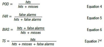
An objective verification approach was employed to measure the models' skill in predicting different weather events. Spatial distribution of model bias against ground observations and GPM measurements for surface temperature and accumulated precipitation were plotted. The bias indicates model accuracy with regard to the observations. Time series for areal average mean error (ME), root mean squared error (RMSE) and Spearman's correlation (CORR) for 2-m temperature and 10-m wind speed were calculated for each model (Equations 1-3).⁶¹ Probability of detection (POD), false alarm rate (FAR), BIAS score and threat score (TS) were computed for 6-hourly accumulated rainfall (Equations 4-7).⁶¹ These statistics were computed for each model at about 200 station points. These are station locations that had valid synops at the forecast hour under investigation (point-to-point verification).

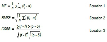
where f is the forecast, o is the observed value, f is the mean forecast and o is the mean observed value.⁶¹

 

Results

Cold Front:15 July 2017

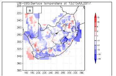
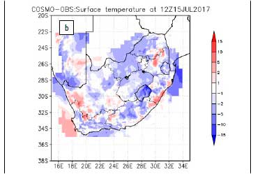
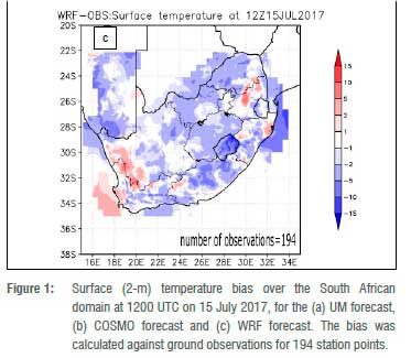
The weather on 15 July 2017 was influenced by a cold front over the southwestern parts of South Africa, preceded by a coastal low along the east coast.⁶² Cold temperatures with snow and heavy rainfall were observed in places over most of the western and southern parts of the country and over the Lesotho highlands.⁵⁹ A synoptic chart that indicates the observations at 12 UTC on the day can be viewed at www.weathersa.co.za/Documents/Publications/20170715.pdf. Figure 1 indicates that the 2-m temperature simulations for the three models have a similar pattern: the models generally have a cold bias. The highest cold bias for all the models is situated over the Lesotho highlands. The UM depicts the highest cold and warm bias (Figure 1a), followed by the COSMO (Figure 1b). The WRF shows the lowest cold and warm bias (Figure 1c). Most of the bias for all the models is within 5 °C of the observed temperatures.

 

 

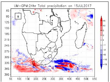
The precipitation that occurred on 15 July 2017 resulted from a cold front over the southwestern parts of South Africa and a coastal low ahead of it. When compared with the GPM measurements, the COSMO model depicts the highest positive bias over South Africa and adjacent oceans (Figure 2b), while the UM (Figure 2a) and WRF (Figure 2c) have a similar pattern. Figure 1a further depicts a negative bias over the southeastern parts of South Africa, implying that the UM failed to capture the precipitation that resulted from a coastal low ahead of the cold front. The COSMO and WRF depict little to no bias in the coastal low area (Figure 2b and 2c). The UM has a larger spatial coverage for positive and negative bias towards the tropics (Figure 2a). The WRF has the lowest positive and negative bias values (Figure 2c).

 

 

The left column in Figure 3 shows the ME, RMSE and CORR for the 2-m temperature for all three models relative to the station observations. The ME for the UM and the WRF closely correspond and generally have a small negative mean bias for most of the day, whereas the COSMO has a much higher positive bias during forecast hours 01-05, and again later in the day (Figure 3). The COSMO model shows almost no temperature bias during forecast hours 09 and 16, because the COSMO has a much larger area over South Africa where warmer temperatures over the northeastern parts of the country were over-forecast and the cooler temperatures over the southern parts were over-forecast, resulting in a small additive bias. The same applies to the early and late hours of the day when the UM and WRF have little to no bias. The UM has the lowest magnitude of errors (RMSE) in the early hours and later in the day when its RMSE is equivalent to the WRF. The RMSE for the three models is almost equivalent during the sunlight hours of the day. The WRF has the lowest correlation during the early hours, but this changes as the three models have equivalent correlation throughout the rest of the diurnal cycle. The model forecasts for 2-m temperature show high correlation with ground observations.

The right column of Figure 3 shows areal average statistics for 10-m wind speed forecasts against ground observations. The three models are comparable. The models have a negative wind speed bias throughout the diurnal cycle. The UM and COSMO have an equivalent bias (ME) throughout the day, while the WRF has lower negative bias in the early hours and higher negative bias later in the day. The models generally have large magnitudes of error (RMSE), and the UM and the COSMO correspond throughout, while the WRF is generally lower in the early hours and higher throughout the rest of the day. The models have low positive correlation for wind speed and it fluctuates throughout the day. The correlation coefficient for WRF is highest during the first two hours when the correlation coefficient for UM and COSMO are very low. The COSMO, sometimes along with the UM, shows the highest correlation coefficient during most sunlight hours, while the WRF has better performance later in the day. Wind forecast skill is poorer than temperature forecasts (Figure 3).

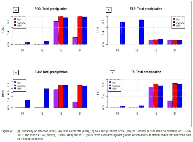
The skill scores for precipitation depict that the precipitation that occurred in the early hours of the day as a result of the coastal low, was only captured by the WRF (Figure 4). A cold front made landfall over the southwestern tip of South Africa later in the day, resulting in significant amounts of rainfall. Only WRF shows skill during the first half of the day, with near perfect bias scores (bias 1) at forecast hour 12 (Figure 4c). Both COSMO and WRF have higher POD during the last half of the day (Figure 4a). At the same time the three models depict equivalent FAR (Figure 4b), the COSMO and WRF show near perfect bias scores (Figure 4c) and higher TS (Figure 4d).

Ridging high and cut-off low: 10 October 2017

The weather on 10 October 2017 was characterised by a cut-off low which is an upper air disturbance that promotes uplift, coupled with a ridging high whose role is the advection of moist air from the ocean onto the land.⁴⁸ A synoptic chart that indicates the observations at 12 UTC on the day can be viewed at www.weathersa.co.za/Documents/Publications/20171010.pdf. Large parts of the southeastern half of South Africa experienced cold temperatures as a result. The models captured these temperatures; however, the extent of the area covered by lower temperatures differs across the three models. The models depict a similar pattern with areas for peak cold and warm biases located at the same points (Figure 5). UM (Figure 5a) and WRF (Figure 5c) are characterised by large areas of cold bias, while the COSMO (Figure 5b) generally over-forecasts surface temperature across the country. WRF depicts the lowest cold and warm bias compared to the other models.

 

 

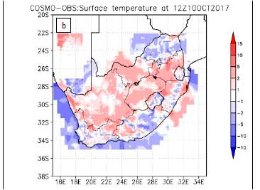
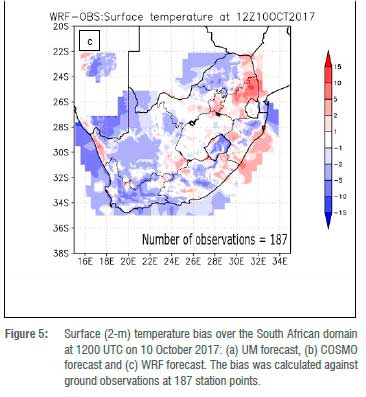
Figure 6 shows the total 24-h precipitation as simulated by the three models compared to GPM rainfall estimates. The spatial coverage and intensities for the three models depict a close resemblance when compared with the GPM measurements (Figure 6). The UM shows the highest positive and negative bias (Figure 6a), followed by COSMO (Figure 6b). The WRF generally depicts the lowest positive and negative bias (Figure 6c).

 

 

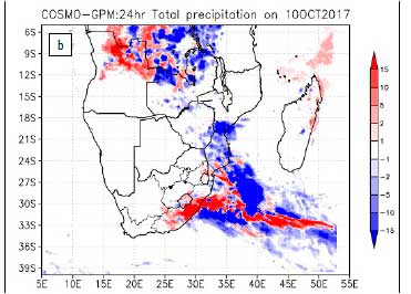
All the models captured the northwest to southeast rainfall pattern, while underestimating the amount in some areas. The rainfall over the southeastern part of South Africa was captured by all the models; however, WRF (Figure 6c) extended the rainfall area more south and north along the coastal area. It may be noted that this event resulted in flooding over the east coast of South Africa, caused severe damage to property and eight people lost their lives.

Surface trough: 30 December 2017

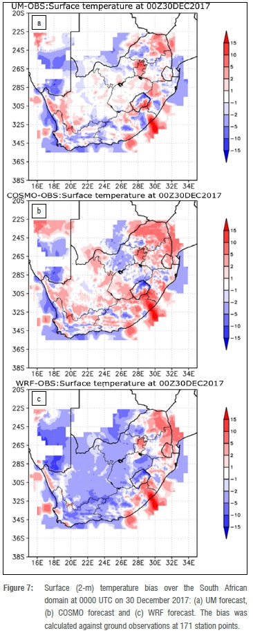
The weather on 30 December 2017 was characterised by a broad surface trough that extended from the central interior to the western parts of South Africa, with a high to the east of the country.⁶⁰ This surface trough resulted in severe thunderstorms associated with a tornado over the central interior of South Africa. A synoptic chart that indicates the observations at 12 UTC on the day can be viewed at www.weathersa.co.za/Documents/Publications/20171230.pdf. The observations at 00 UCT on 30 December 2017 were characterised by cooler temperatures across most of the eastern and southern parts of the country. A warm tongue was observed in the Northern Cape which extends into Namibia. The three models were able to capture the general spatial pattern showing lower temperatures over the south and east of the country. The models' simulations depict a similar pattern for surface temperature simulations with peaks for cold and warm biases situated at the same locations (Figure 7). The UM and COSMO generally show a positive bias (Figure 7a,b). WRF depicts larger areas of cold bias within 5 °C.

 

 

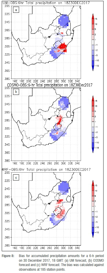
A large band of rainfall, extending from the tropics to the southern coast of South Africa, was observed on 30 December 2017. The 6-hourly accumulated precipitation for models compared with ground observations were used in this case as they contain more detail than the 24-hour totals. All the time steps followed a similar pattern, hence one time step is depicted. The models depict a similarity in simulating precipitation (Figure 8). The UM depicts the highest positive and negative biases, followed by WRF.

 

 

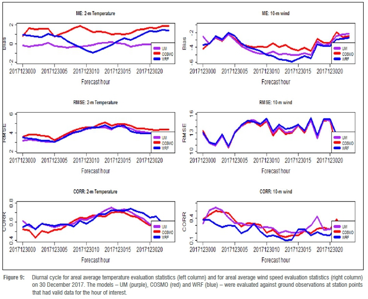
Additive bias for 2-m temperature shows high accuracy for the UM throughout the day (Figure 9, left column). There is a general over-forecast by the COSMO throughout the day. The WRF shows an over-forecast in the early and late hours, and a gradual decline during sunlight hours, to as low as -1 towards midday. The models have equivalent magnitudes of error (RMSE) for temperature throughout the diurnal cycle. The correlation coefficient for the models is also equivalent, although it is low.

The right column of Figure 9 shows statistics for 10-m wind speed. The models under-forecast wind speed throughout the diurnal cycle, and they have equivalent ME, except during the warm hours of the day when the COSMO simulation is relatively more accurate. The models show equivalent RMSE throughout the diurnal cycle. The models show a low correlation throughout the diurnal cycle.

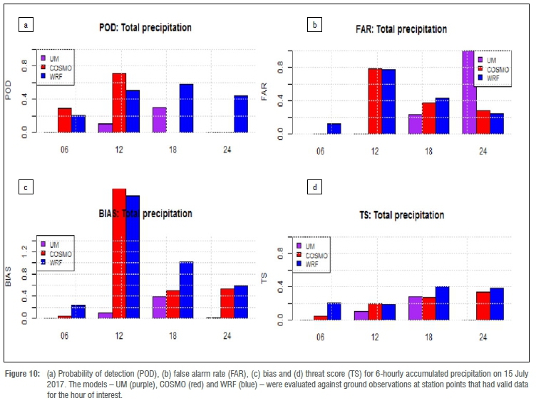
The POD for precipitation at station points over South Africa is higher for the COSMO during the first half of the day, and higher for the WRF for the rest of the day (Figure 10). The WRF has the highest FAR at forecast hours 06 and 18, while the COSMO has the highest at forecast hour 12 and UM at forecast hour 24. The UM under-forecasts precipitation throughout the diurnal cycle. The WRF shows relatively high accuracy throughout (bias closest to the perfect score of 1); although the models have low TS throughout the diurnal cycle, WRF shows better skill compared to the other models.

 

Discussions and conclusions

In this study, we evaluated the performance of three models, used within the SADC region for operational weather forecasting in South Africa, in simulating three high-impact weather events. These three events were associated with a cold front, a ridging high associated with an upper-air cut-off low, and a surface trough and tornado, respectively. The second event resulted in flooding over parts of the east coast of South Africa with eight people reported to have lost their lives. The third event was reported to have damaged houses in parts of the central interior of South Africa. All three models were able to capture the events, with slight differences in performance.

All the models were able to capture the general temperature pattern with an acceptable areal average bias of about 1 °C. COSMO generally underestimated the size of the area associated with lower temperatures. The three models generally underestimated the temperature in the Limpopo Province, especially in the western parts of the province. The models failed to capture warmer temperatures over the western interior of South Africa that extended into Namibia. WRF captured this feature best; however, the area was overestimated. The three models poorly simulated 10-m winds, and as a result produced high bias and poorly correlated with ground observations.

The three models were able to capture the general rainfall pattern associated with the three case studies: 24-h accumulated precipitation for the three models was comparable to the observations, while 6-h accumulated rainfall showed poor performance. This is most noticeable on 30 December 2017 where FAR is high and POD is poor. The spatial pattern of the rainfall differed across the three models and, in some instances, the WRF and the COSMO underestimated the rainfall amount. The COSMO did not capture all the rainfall associated with the rain bands that extended from the tropics to South Africa in a northwest to southeast pattern on 10 October 2017 and 30 December 2017.

WRF was able to capture rainfall associated with the coastal low better than the other two models. COSMO captured the event, but underestimated the rainfall, while the UM did not capture the event at all. The UM generally depicted a similar or higher amount of rainfall as that observed, but had a much smaller spatial coverage (blobbiness). COSMO generally failed to capture small and residual rainfall, and also forecasted slightly lower amounts of rainfall than the GPM observations. WRF performed well over land, and even captured the small (and residual) rainfall that the UM and COSMO did not capture. However, it overestimated rainfall over the ocean.

The study shows that the models are skilled in capturing general details of big events, similar to the ones that were analysed here. The differences in the simulations point to issues with small-scale processes and, in particular, in the simulation of rainfall. The poor performance of the models may be associated with the use of coarse-resolution observations and non-gridded data sets.^1,63 It is important that further research is conducted to understand the reasons associated with the different model performances. However, it may be noted, as also shown in this study, that there are shortcomings in the available observations, which makes it difficult for models to be verified in detail. Satellite estimates show different amounts of rainfall, as also shown here.

 

Acknowledgements

We are grateful for a Climate Research for Development (CR4D) fellowship grant (reference number CR4D-19-11), managed by the African Academy of Sciences. We also thank the South African National Integrated Cyber-Infrastructure System (NICIS), Centre for High Performance Computing (CHPC), for the computational resources as well as model set-up, and Germany's national meteorological service, the Deutscher Wetterdienst, for helping with the COSMO model set-up.

 

Competing interests

We have no competing interests to declare.

 

Authors' contributions

PT.M.: Conceptualisation, methodology, data collection, data analysis and validation, data curation, writing - the initial draft. G.T.R.: Methodology, data analysis and validation, data curation, writing - the initial draft. M-J.B.: Methodology, data collection, data analysis and validation, data curation, funding acquisition, writing - the initial draft. R.M.: Writing -the initial draft. N.M.: Data curation.

 

References

1. Clark P Roberts N, Lean H, Ballard SP Charlton-Perez C. Convection-permitting models: A step-change in rainfall forecasting. Meteorol Appl. 2016;23:165-181. https://doi.org/10.1002/met.1538        [ Links ]

2. Bauer P Thorpe A, Brunet G. The quiet revolution of numerical weather prediction. Nature. 2015;525:47-55. https://doi.org/10.1038/nature14956        [ Links ]

3. Schultze GC. Atmospheric observations and numerical weather prediction. S Afr J Sci. 2007;103(7-8):318-323.         [ Links ]

4. Duan Q, Di G, Quan J, Wang C, Gong W. Automatic model calibration: A new way to improve numerical weather forecasting. Bull Am Meteorol Soc. 2017;98(5):959-970. https://doi.org/10.1175/BAMS-D-15-00104.1        [ Links ]

5. Schättler U, Doms U, Schraff C. A Description of the nonhydrostatic regional COSMO-model. Offenbach: Deutscher Wetterdienst; 2014.         [ Links ]

6. Tang Y, Lean WH, Bornemann J. The benefits of the Met Office variable resolution NWP model for forecasting convection. Meteorol Appl. 2013;20:417-126. https://doi.org/10.1002/met.1300        [ Links ]

7. Maisha TR. The influence of topography and grid resolution on extreme weather forecasts over South Africa [thesis]. Pretoria: University of Pretoria; 2014.         [ Links ]

8. Dabernig M, Mayr GJ, Messner JW. Predicting wind power with reforecasts. Weather Forecast. 2015;30:1655-1662. https://doi.org/10.1175/WAF-D-15-0095.1        [ Links ]

9. Peel MC, Finlayson BL, McMahon TA. Updated world map of the Köppen-Geiger climate classification. Hydrol Earth Syst Sci. 2007;11:1633-1644. https://doi.org/10.5194/hess-11-1633-2007        [ Links ]

10. Daron JD. Regional climate messages: Southern Africa. Scientific report from the CARIIA Adaptation at Scale in Semi-Arid Regions (ASSAR) Project. Ottawa: CARIAA and ASSAR; 2014.         [ Links ]

11. Engelbrecht CJ, Engelbrecht FA. Shifts in Köppen-Geiger climate zones over southern Africa in relation to key global temperature goals. Theor Appl Climatol. 2016;123:247-261. https://doi.org/10.1007/s00704-014-1354-1        [ Links ]

12. Dong B, Gregory JM, Sutton RT. Understanding land-sea warming contrast in response to increasing greenhouse gases. Part I: Transient adjustment. J Clim. 2009;22:3079-3097. https://doi.org/10.1175/2009JCLI2652.1        [ Links ]

13. Liou KN. Radiation and cloud processes in the atmosphere: Theory, observation and modeling. London: Oxford University Press; 1992.         [ Links ]

14. Sellers PJ. Biophysical models of land surface processes. In: Trenberth K, editor. Climate system modeling. Cambridge, UK: Cambridge University Press; 1993.         [ Links ]

15. Krishnamurti TN, Bounoua L. An introduction to numerical weather prediction techniques. Boca Raton, FL: CRC Press; 1996. https://doi.org/10.1201/9781315137285        [ Links ]

16. Saur D. Evaluation of the accuracy of numerical weather prediction models. In: Silhavy R, Senkerik R, Oplatkova Z, Prokopova Z, Silhavy P editors. Artificial intelligence perspectives and applications. Advances in intelligent systems and computing vol 347. Cham: Springer; 2015. https://doi.org/10.1007/978-3-319-18476-0_19        [ Links ]

17. Mahlobo DD. The verification of different model configurations of the Unified Atmospheric Model over South Africa [thesis]. Pretoria: University of Pretoria; 2013.         [ Links ]

18. Kann A, Wittmann C, Bica B, Wastl C. On the impact of NWP model background on very high-resolution analysis in complex terrain. Weather Forecast. 2015;30(4):1077-1089. https://doi.org/10.1175/WAF-D-15-000L1        [ Links ]

19. Baldauf M, Seifert A, Forster J, Majewski D, Raschendorfer M, Reinhardt T. Operational convective-scale numerical weather prediction with the COSMO model: Description and sensitivities. Mon Weather Rev. 2011;139(12):3887-3904. https://doi.org/10.1175/MWR-D-10-05013.1        [ Links ]

20. Mulovhedzi P. Towards a heat-watch warning system for South Africa for the benefit of the health sector [thesis]. Pretoria: University of Pretoria; 2017.         [ Links ]

21. Woodhams BB. What is the added value of a convection-permitting model for forecasting extreme rainfall over tropical East Africa? Mon Weather Rev. 2018;146:2757-2780. https://doi.org/10.1175/MWR-D-17-0396.1        [ Links ]

22. Stein THM, Keat W, Maidment RI, Landman S, Becker E, Boyd DFA, et al. An evaluation of clouds and precipitation in convection-permitting forecasts for South Africa. Weather Forecast. 2019;34(1):233-254. https://doi.org/10.1175/WAF-D-18-0080.1        [ Links ]

23. Schmidli J, Billings B, Chow F, De Wekker S, Doyle J, Grubisic V et al. Intercomparison of mesoscale model simulations of the daytime valley wind system. Mon Weather Rev. 2011;139:1389-1409. https://doi.org/10.1175/2010MWR3523.1        [ Links ]

24. Bopape M-JM, Sithole HM, Motshegwa T, Rakate E, Engelbrecht F, Archer E, et al. A regional project in support of the SADC Cyber-Infrastructure Framework Implementation: Weather and climate. Data Sci J. 2019;18:1-10. https://doi.org/10.5334/dsj-2019-034        [ Links ]

25. Doms G, Baldauf M. A description of the nonhydrostatic regional COSMO-model. Part I: Dynamics and numerics. Offenbach: Deutscher Wetterdienst; 2018.         [ Links ]

26. Davies T, Cullen MJP, Malcolm AJ, Mawson MH, Staniford A, White AA, et al. A new dynamical core for the Met Office's global and regional modelling of the atmosphere. Q J Roy Meteor Soc. 2005;131:1759-1782. https://doi.org/10.1256/qj.04.101        [ Links ]

27. Greed G, Haywood JM, Milton S, Keil A, Christopher S, Gupta P et al. Aerosol optical depths over North Africa 2: Modeling and model validation. J Geophys Res. 2008;113:D00C05. https://doi.org/10.1029/2007JD009457        [ Links ]

28. Manners J, Vosper SB, Roberts N. Radiative transfer over resolved topographic features for high-resolution weather prediction. Q J Roy Meteor Soc. 2012;138:720-733. https://doi.org/10.1002/qj.956        [ Links ]

29. Edwards JM, Slingo A. Studies with a flexible new radiation code. I: Choosing a configuration for a largescale model. Q J Roy Meteor Soc. 1996;122:689-719. https://doi.org/10.1002/qj.49712253107        [ Links ]

30. Wilson DR, Ballard SPP A micro-physically based precipitation scheme for the UK Meteorological Office Unified Model. Q J Roy Meteor Soc. 1999;125:1607-1636. https://doi.org/10.1002/qj.49712555707        [ Links ]

31. Abel SJ, Shipway BJ. A comparison of cloud-resolving model simulations of trade wind cumulus with aircraft observations taken during RICO. Q J Roy Meteor Soc. 2007;133:781-794. https://doi.org/10.1002/qj.55        [ Links ]

32. Khairoutdinov M, Kogan Y A new cloud physics parameterization in a large-eddy simulation model of marine stratocumulus. Mon Weather Rev. 2000;128:229-243. https://doi.org/10.1175/1520-0493(2000)128<0229:ANCPPI>2.0.CO;2        [ Links ]

33. Boutle IA, Abel SJ, Hill PG, Morcrette CJ. Spatial variability of liquid cloud and rain: Observations and microphysical effects. Q J Roy Meteor Soc. 2014;140:583-594. https://doi.org/10.1002/qj.2140        [ Links ]

34. Field PR, Hogan RJ, Brown PRA, Illingworth AJ, Choularton TW, Cotton RJ. Parametrization of ice-particle size distributions for mid-latitude stratiform cloud. Q J Roy Meteor Soc. 2005;13:1997-2017. https://doi.org/10.1256/qj.04.134        [ Links ]

35. Gregory D, Rowntree PR. A mass-flux convection scheme with representation of cloud ensemble characteristics and stability dependent closure. Mon Weather Rev. 1990;118:1483-1506. https://doi.org/10.1175/1520-0493(1990)118<1483:AMFCSW>2.0.CO;2        [ Links ]

36. Lock AP Brown AR, Bush MR, Martin GM, Smith RNB. A new boundary layer mixing scheme. Part I: Scheme description and single-column model tests. Mon Weather Rev. 2000;128:3187-3199. https://doi.org/10.1175/1520-0493(2000)128<3187:ANBLMS>2.0.CO;2        [ Links ]

37. Best MJ, Pryor M, Clark DB, Rooney GG, Essery RLH, Ménard CB, et al. The Joint UK Land Environment Simulator (JULES), model description - Part 1: Energy and water fluxes. Geosci Model Dev. 2011;4:677-699. https://doi.org/10.5194/gmd-4-677-2011        [ Links ]

38. Clark DB, Mercado LM, Sitch S, Jones CD, Gedney N, Best MJ, et al. The Joint UK Land Environment Simulator (JULES), model description - Part 2: Carbon fluxes and vegetation dynamics. Geosci Model Dev. 2011;4:701-722. https://doi.org/10.5194/gmd-4-701-2011        [ Links ]

39. Tiedtke M. A comprehensive mass flux scheme for cumulus parameterization in large-scale models. Mon Weather Rev. 1989;117:1779-1799. https://doi.org/10.1175/1520-0493(1989)117<1779:ACMFSF>2.0.CO;2        [ Links ]

40. Doms G, Förstner J, Heise E, Herzog H-J, Mironov D, Raschendorfer M, et al. A description of the nonhydrostatic regional COSMO model. Part II: Physical parameterization. Offenbach: Deutscher Wetterdienst; 2018.         [ Links ]

41. Ritter B, Geleyn J-F. A comprehensive radiation scheme for numerical weather prediction models with potential applications in climate simulations. Mon Weather Rev. 1992;120:303-325. https://doi.org/10.1175/1520-0493(1992)120<0303:ACRSFN>2.0.CO;2        [ Links ]

42. Jacobsen I, Heise E. A new economic method for the computation of the surface temperature in numerical models. Contr Atmos Phys.1982;55:128-141.         [ Links ]

43. Arakawa A, Moorthi S. Baroclinic instability in vertically discrete systems. J Atmos Sci. 1988;45(11):1688-1708. https://doi.org/10.1175/1520-0469(1988)045<1688:BIIVDS>2.0.CO;2        [ Links ]

44. Wicker L, Skamarock W. Time-splitting methods for elastic models using forward time schemes. Mon Weather Rev. 2002;130:2088-2097. https://doi.org/10.1175/1520-0493(2002)130<2088:TSMFEM>2.0.CO;2        [ Links ]

45. Mironov D. Parameterization of lakes in numerical weather prediction. Description of a lake model. COSMO Technical report no. 11. Offenbach: Deutscher Wetterdienst; 2008.         [ Links ]

46. Mironov D, Ritter B. Testing the new ice model for the global NWP system GME of the German Weather Service. In: Cote J, editor. Research activities in atmospheric and oceanic modelling. Rep. 34 WMO/TD 1220 4.21-4.22. Geneva: World Meteorological Organization; 2004.         [ Links ]

47. Schulz J-P Introducing a sea ice scheme in the COSMO model. COSMO Newsletter. 2011;11:32-40.         [ Links ]

48. Skamarock WC, Klemp JB, Dudhia J, Gill DO, Barker DM, Duda MG, et al. A description of the advanced research WRF version 3. NCAR Technical note NCAR/TN-475+STR. Boulder, CO: Mesoscale and Microscale Meteorology Division, National Center for Atmospheric Research; 2008. https://doi.org/10.5065/D68S4MVH        [ Links ]

49. Hong SY Lim OJ. The WRF single-moment 6-class microphysics scheme (WSM6). J Korean Meteor Soc. 2006;42:129-151.         [ Links ]

50. lacono MJ, Delamere JS, Mlawer EJ, Shephard MW, Clough SA, Collins WD. Radiative forcing by long-lived greenhouse gases: Calculations with the AER radiative transfer models. J Geophys Res. 2008;113:D13103. https://doi.org/10.1029/2008JD009944        [ Links ]

51. Hong S-Y Noh Y Dudhia J. A new vertical diffusion package with an explicit treatment of entrainment processes. Mon Weather Rev. 2006;134:2318-2341. https://doi.org/10.1175/MWR3199.1        [ Links ]

52. Skamarock WC, Klemp JB, Dudhia J, Gill DO, Liu Z, Berner J, et al. A Description of the advanced research WRF version 4. NCAR Technical note NCAR/TN-556+STR. Boulder, CO: Mesoscale and Microscale Meteorology Division, National Center for Atmospheric Research; 2019.         [ Links ]

53. US National Aeronautics and Space Administration (NASA). Global Precipitation Measurement, GPM Data Downloads [webpage on the Internet]. No date [cited 2018 Jul 20]. Available from: https://gpm.nasa.gov/data-access/downloads/gpm        [ Links ]

54. Skofronick-Jackson G, Petersen WA, Berg W, Kidd C, Stocker EF, Kirschbaum DB, et al. The Global Precipitation Measurement (GPM) Mission for science and society. Bull Am Meteorol Soc. 2017; 98:1679-1695. https://doi.org/10.1175/BAMS-D-15-00306.1        [ Links ]

55. Retalis A, Katsanos D, Tymvios D, Michaeli S. Comparison of GPM IMERG and TRMM 3B43 products over Cyprus. Remote Sens. 2020;12:3212. https://doi.org/10.3390/rs12193212        [ Links ]

56. Dezfuli AK, Ichoku CM, Huffman GJ, Mohr Kl, Selker JS, Van de Giesen N, et al. Validation of IMERG precipitation in Africa. J Hydrometeorol. 2017;18:2817-2825. https://doi.org/10.1175/JHM-D-17-0139.1        [ Links ]

57. Suleman S, Chetty KT, Clark DJ, Kapangaziwiri E. Assessment of satellite-derived rainfall and its use in the ACRU agro-hydrological model. Water SA. 2020;46(4):547-557. https://doi.org/10.17159/wsa/2020.v46.i4.9068        [ Links ]

58. Muofhe T, Chikoore H, Bopape M-J, Nethengwe N, Ndarana T, Rambuwani GT. Forecasting intense cut-off lows in South Africa using the 4.4 km Unified Model. Climate. 2020;8:129. https://doi.org/10.3390/cli8110129        [ Links ]

59. Snow Report SA. The history of snow in southern Africa [webpage on the Internet]. No date [cited 2019 June 24]. Available from: https://snowreport.co.za/history-of-snow-in-south-africa-after-2010        [ Links ]

60. Gordon N, Shaykewich J. Guidelines on performance assessment of public weather services. WMO/TD No.1023. Geneva: World Meteorological Organization; 2000.         [ Links ]

61. Sass BH, Yang X. A verification score for high resolution NWP: Idealized and preoperational tests. HIRLAM Technical report no. 69. De Bilt: KNMI; 2012.         [ Links ]

62. South African Weather Service (SAWS). Caelum: Notable weather and weather-related events in 2017. Pretoria: SAWS; 2018.         [ Links ]

63. Champion AJ, Hodges K. Importance of resolution and model configuration when downscaling extreme precipitation. Tellus A. 2014;66:23993. https://doi.org/10.3402/tellusa.v66.23993        [ Links ]

 

 

Correspondence:
Patience Mulovhedzi
Email: patience.mulovhedzi@weathersa.co.za

Received: 13 July 2020
Revised: 08 Jan. 2021
Accepted: 28 Feb. 2021
Published: 29 Sep. 2021

 

 

Funding: African Academy of Sciences Climate Research for Development (grant no. CR4D-19-11)
Editor: Yali Woyessa