RESEARCH ARTICLE

 

Predicting take-up of home loan offers using tree-based ensemble models: A South African case study

 

 

Tanja Verster^I; Samistha Harcharan^II; Lizette Bezuidenhout^III; Bart Baesens^IV

^ICentre for Business Mathematics and Informatics, North-West University, Potchefstroom, South Africa
^IIModel Risk, First National Bank, Johannesburg, South Africa
^IIIModel Risk, Absa, Johannesburg, South Africa
^IVDepartment of Decision Sciences and Information Management, KU Leuven University, Leuven, Belgium

Correspondence

 

 

---

ABSTRACT

We investigated different take-up rates of home loans in cases in which banks offered different interest rates. If a bank can increase its take-up rates, it could possibly improve its market share. In this article, we explore empirical home loan price elasticity, the effect of loan-to-value on the responsiveness of home loan customers and whether it is possible to predict home loan take-up rates. We employed different regression models to predict take-up rates, and tree-based ensemble models (bagging and boosting) were found to outperform logistic regression models on a South African home loan data set. The outcome of the study is that the higher the interest rate offered, the lower the take-up rate (as was expected). In addition, the higher the loan-to-value offered, the higher the take-up rate (but to a much lesser extent than the interest rate). Models were constructed to estimate take-up rates, with various modelling techniques achieving validation Gini values of up to 46.7%. Banks could use these models to positively influence their market share and profitability.
SIGNIFICANCE:
• We attempt to answer the question: What is the optimal offer that a bank could make to a home loan client to ensure that the bank meets the maximum profitability threshold while still taking risk into account? To answer this question, one of the first factors that needs to be understood is take-up rate. We present a case study - with real data from a South African bank - to illustrate that it is indeed possible to predict take-up rates using various modelling techniques.

Keywords: pricing, retail credit risk, boosting, bagging, price elasticity

---

 

 

Introduction

On a daily basis, banks receive home loan applications from potential customers. Depending on the customer's risk profile, affordability and other factors, the bank decides whether or not to offer a home loan to this customer. The risk profile and affordability dictate the interest rate and which loan amount (relative to the value of the house) will be offered. The take-up of these offered home loans influences the profit of a bank. If more customers take-up the offers, the profit can potentially increase (i.e. the bank's market share might increase) and if customers do not take-up these offers, the bank cannot potentially increase profit and market share. However, if more high-risk customers take up these offers, the bank might lose money due to customers defaulting. If low-risk customers decline these offers, the bank loses potential income. By understanding the factors that influence the take-up rates of home loans offered, the bank potentially benefits through increased market share and profits. In this paper, we build a model to predict the probability of take-up of home loans offered by focusing on interest rate¹ and loan-to-value (LTV)². This take-up model relates to the responsiveness of a specific customer segment (based on, for example, the risk type of a customer) to a change in the quoted price. The 'price' of a home loan is the interest rate charged by a bank to the customer.

Banks improve their market share (and possibly also profitability) when they increase the take-up rate by offering different interest rates ('price') to different customers using risk-based pricing. To determine which interest rate to charge and for which customer, the bank needs to understand the risk levels and price elasticity of a customer; that is, how sensitive the customer is to interest rate changes. For example, at a price of 10%, a bank might sell the credit product (home loan) to 100 customers, yet at a price of 11% it would only sell to 90 customers. This emphasises the importance of understanding 'take-up probability' (also referred to as the 'price-response function').

The aim of this paper is threefold. Firstly, we investigate price elasticity on a South African home loan data set. To investigate the effect of only interest rate on take-up, we will build a logistic regression using only one covariate (i.e. interest rate). Secondly, we illustrate the effect of LTV on take-up rates in South Africa. Again, to illustrate this, a logistic regression is built using only LTV as the covariate. Lastly, we investigate whether it is possible to predict take-up rates of home loans offered by a bank using a combination of LTV and interest rates. Both logistic regression and tree-ensemble models were considered.

We focused primarily on the effect of interest rates and LTV on the take-up rates. Note that take-up rates are also influenced by other factors such as competitor offers, where another bank offers a home loan with more attractive terms (e.g. lower interest rate and higher LTV), which could hugely influence the take-up rate. Another factor is the turnaround time of an application, where a customer applies for a home loan at two different banks with similar loan terms. The bank that processes the application more swiftly is more likely to be accepted by the customer than the bank that takes longer to process the application.¹ These factors were not taken into account in this paper.

 

Interest rates and LTV

Our focus in this paper is to investigate how interest rates and LTV influence take-up rates of home loans. A fundamental quantity in the analysis of what price to set for any product, is the price-response function - how much the demand for a product varies as the price varies. This is the probability that a customer will take up the offer of a home loan. We will distinguish between take-up and non-take-up - the customer accepting (take-up) or not accepting (non-take-up) the home loan from the bank. As in Thomas¹, we will also use the terms 'take-up probability' and 'price-response function' interchangeably. The simplest price-response function is the linear function, but the more realistic price-response function is the logit function.¹ Within the retail credit environment, relatively little has been published about price elasticity, even though price elasticity is a well-known concept in other fields.

The effect of interest rates on take-up rates is also referred to as price elasticity. Phillips³ outlines a number of reasons why the same product (e.g. a home loan) can be sold at different prices. Note that from the bank's viewpoint, banks typically 'price' for risk by charging a higher interest rate for higher-risk customers. From the customer's viewpoint, however, banks can also 'price' their loan product at different interest rates to increase market share (and possibly profitability).⁴ Specifically, price elasticity can be seen as the willingness of a customer to pay for a product or service.^1,5 Pricing is a strategic tool⁶ for acquiring new customers and retaining existing ones⁷. Limited studies of price elasticity have been done in emerging countries such as South Africa, for example the study on personal loans⁵ and the study on micro-loans⁸. Very little research has been conducted on the price elasticity of home loans, both locally and internationally. In this paper, we investigate price elasticity on a specific home loan portfolio of a South African bank.

LTV is considered to be one of the most important factors in home loans lending - the higher the LTV, the higher the risk is from the bank's point of view.^2,9,10 The LTV ratio is a financial term used by lenders to express the ratio of a loan compared to the value of an asset purchased. In a paper by Otero-González, et al.², the default behaviour (risk) of home loan customers is explained using the LTV ratio. The influence of LTV on take-up rates is a 'chicken-and-egg' conundrum. The LTV offered to a customer will influence their take-up rate, but the LTV also influences the risk of the customer and their ability to repay the loan - the higher the LTV, the higher the risk of the bank losing money, as the sale of the property might not cover the home loan. On the other hand, the LTV offered to a customer is determined by the risk of the customer.¹¹ The bank will consider the risk of the customer to determine what LTV to offer, that is, a higher-risk customer will qualify for a lower LTV in order to prevent over-extending credit to the customer.

The same is true for interest rates. The interest rate offered to the customer influences take-up rates. However, the risk of a customer determines the interest rate offered to that customer, and the interest rate offered to the customer then influences the risk. The higher the interest rate, the higher the monthly repayment, which affects the affordability to a customer and thereby influences the risk of the customer.

 

Modelling take-up rates

The last aim of this paper is to predict take-up of home loans offered using logistic regression as well as tree-based ensemble models.

Logistic regression is commonly used to predict take-up rates.⁵ Logistic regression has the advantages of being well known and relatively easy to explain, but sometimes has the disadvantage of potentially underperforming compared to more complex techniques.¹¹ One such complex technique is tree-based ensemble models, for example bagging and boosting.¹² Tree-based ensemble models are based on decision trees.

Decision trees, also more commonly known as classification and regression trees (CART), were developed in the early 1980s.¹³ Decision-tree models have several advantages¹⁴ - among others, they are easy to explain and can handle missing values. Disadvantages include their instability in the presence of different training data and the challenge of selecting the optimal size for a tree. Two ensemble models that were created to address these problems are bagging and boosting. We use these two ensemble algorithms in this paper.

Ensemble models are the product of building several similar models (e.g. decision trees) and combining their results in order to improve accuracy, reduce bias, reduce variance and provide robust models in the presence of new data.¹⁴ These ensemble algorithms aim to improve accuracy and stability of classification and prediction models.¹⁵ The main difference between these models is that the bagging model creates samples with replacement, whereas the boosting model creates samples without replacement at each iteration.¹² Disadvantages of model ensemble algorithms include the loss of interpretability and the loss of transparency of the model results.¹⁵

Bagging applies random sampling with replacement to create several samples. Each observation has the same chance to be drawn for each new sample. A decision tree is built for each sample and the final model output is created by combining (through averaging) the probabilities generated by each model iteration.¹⁴

Boosting performs weighted resampling to boost the accuracy of the model by focusing on observations that are more difficult to classify or predict. At the end of each iteration, the sampling weight is adjusted for each observation in relation to the accuracy of the model result. Correctly classified observations receive a lower sampling weight, and incorrectly classified observations receive a higher weight. Again, a decision tree is built for each sample and the probabilities generated by each model iteration are combined (averaged).¹⁴

In this paper, we compare logistic regression against tree-based ensemble models. As mentioned, tree-based ensemble models offer a more complex alternative to logistic regression with a possible advantage of outperforming logistic regression.¹²

In the process of determining how well a predictive modelling technique performs, the lift of the model is considered, where lift is defined as the ability of a model to distinguish between the two outcomes of the target variable (in this paper, take-up vs non-take-up). There are several ways to measure model lift¹⁶; in this paper, the Gini coefficient was chosen, similar to measures applied by Breed and Verster¹⁷. The Gini coefficient quantifies the ability of the model to differentiate between the two outcomes of the target variable.^16,18 The Gini coefficient is one of the most popular measures used in retail credit scoring.^1,19,20 It has the added advantage of being a single number between 0 and 1.¹⁶

 

Scenario setting

In the South African market, home loans are typically offered over a period of 20 to 30 years. If an application passes the credit vetting process (an application scorecard as well as affordability checks), an offer is made to the client detailing the loan amount and interest rate offered. Both the deposit required as well as the interest rate requested are a function of the estimated risk of the applicant and the type of finance required.

Ordinary home loans, building loans as well as top-up loans (a further advance on a home loan) are different types of loans offered in the retail sector.²¹ The value of the property is obtained from a central automated valuation system accessed by all mortgage lenders.²² Where an online valuation is not available, the property will be physically evaluated. Depending on the lender's risk appetite, a loan of between 60% and 110% of the property valuation will be offered to the applicant and is the LTV. The prime lending rate is the base rate that lenders use to make the offer, for example prime plus 2 or prime less 0.5. Mortgage loans are normally linked to interest rates and can fluctuate over the repayment period.²³ Fixed interest rates are normally only offered on short-term unsecured loans. The repurchase rate (repo rate) is determined by the South African Reserve Bank (Central Bank) Monetary Committee and is the rate at which the Central Bank will lend to the commercial banks of South Africa.²⁴ The prime rate is a direct function of the repo rate.

In all analyses, we subtract the repo rate from the interest rate to remove the effect of the fluctuations due to the fiscal policy that is reflected by the repo rate. This ensures that our analysis is not affected by the specific level of interest rate in South Africa. The analysis is done on the percentage above or below the repo interest rate. Note that as South Africa is a developing country, the repo rate fluctuates more frequently than it does in developed economies.

The sample consisted of 294 479 home loan approvals from one South African bank, with offers between January 2010 and July 2015. From these offers, 70% were taken up by the applicants for the varying LTVs and interest rates. The type of data available for each customer are:

• General demographic information gathered at application (e.g. income, gender, employment type).

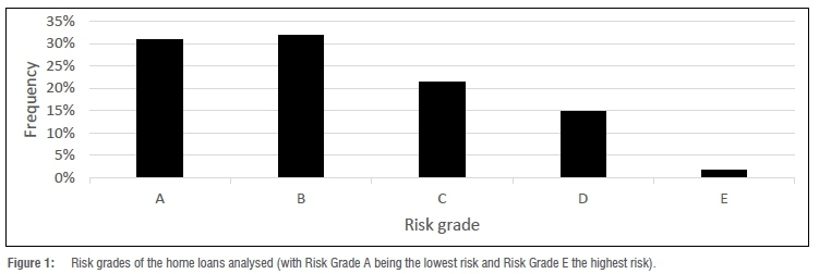
• The application risk grade (the result of a home loan application scorecard resulting in five risk grades, with Risk Grade A being the lowest risk and Risk Grade E the highest risk).

• Information about the home loan offered (e.g. interest rate offered in terms of repo rate, the LTV, the term, type of loan i.e. building loan (B), further advance building loan (FAB), further advance ordinary loan (FAO), ordinary home loan (O); and an indicator as to whether the customer was new to this bank's home loan or not).

The risk grades are provided in Figure 1. The left side of Figure 1 indicates the lowest risk (Risk Grade A) and the right indicates the highest risk (Risk Grade E). The risk grade is usually derived from the results of a credit scorecard.^20,25

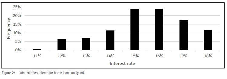
Figure 2 shows the interest rates offered. Note that in Figure 2 the interest rate is adjusted by subtracting the repo rate.

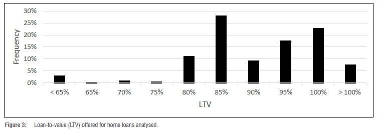
The LTV offered is illustrated in Figure 3. A lower value of LTV indicates that the home loan value is less than the property value (i.e. 50% < LTV < 100%) and a higher value of LTV is where the home loan value is higher than the property value (i.e. LTV > 100%). An LTV higher than 100% can include additional costs (e.g. transfer cost), which is usually allowed for first-time buyers.

 

Price elasticity: Interest rate effect on take-up rates

To investigate the sensitivity of take-up to a change in the interest rate offered, a logistic regression was built. First, the data were split²⁶ into a training data set (70% or 205 802 observations) and a validation data set (30% or 88 677 observations), keeping the 30% non-take-up and 70% take-up rates in both data sets¹⁸, in other words, stratified sampling²⁷. The following data preparations were performed: subtract the repo rate from the interest rate; change class variables to numeric variables (using indicator functions); and scale certain variables (e.g. divide by 10 000).

A logistic regression model was built to predict a take-up rate given a certain interest rate (or LTV) offered. The probability of take-up is defined as the number of customers taking up a home loan divided by the number of customers who were offered a home loan. Note that the interest rate (and LTV) is an iterative process due to affordability (this relates to the chicken-and-egg conundrum). The resulting logistic regression is the price-response function. As mentioned before, a realistic price-response function is the logit function and therefore a logistic regression works very well in this context.

Using 5.5 years' of home loan data, a logistic regression was fitted on the interest rate:

where 0=β₀+β₁ X₁%, and p is the probability of take-up and where X₁ is the recommended interest rate offered to the customer.

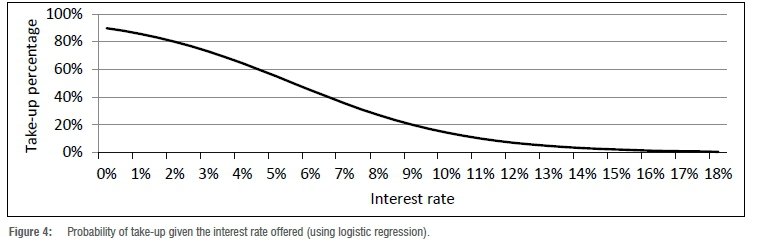
Due to confidentiality, the details of the estimates (β₀, β₁) are not given, but the logistic regression equation (p) is plotted in Figure 4. The Gini coefficient on the training data set was 0.316 and on the validation data set it was 0.314. The 95% confidence interval on the Gini coefficient on the validation data set was determined as (0.307; 0.322).

Figure 4 clearly shows that price elasticity exists in the home loans portfolio. The higher the interest rate offered, the lower the take-up rate. The take-up rates vary between 0% (very high interest rates) and 90% (very low interest rates offered). This illustrates the acceptance of loans that vary with the level of interest rate offered.

 

Interest rate effect on take-up rates: Different risk grades

We now investigate whether the price elasticity curves are the same for 'good' and 'bad' customers.

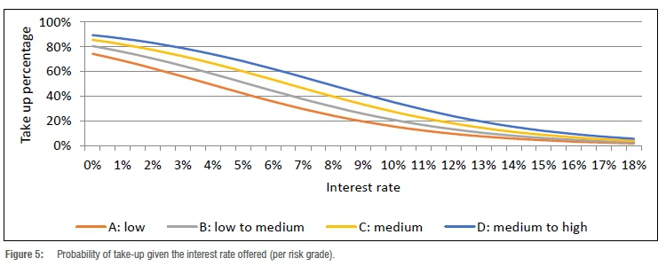
The logistic regression equation fitted to both the risk grade and interest rate shows that customers with medium to high risk - in other words, 'bad' customers - are less sensitive to rate changes than customers with low risk who are considered 'good' customers, as depicted in Figure 5. This shows that the take-up rate is higher for 'bad' customers versus 'good' customers for a given interest rate.

 

LTV effect on take-up rates

We now investigate how sensitive home loan customers are to the LTV offered. Again, note that the LTV is determined greatly by the risk of the customer as well as the size of the loan.

The following logistic regression was fitted:

where 0=β₀+β₂ (X₂) and p is the probability of take-up and where X₂ is the LTV calculated by the LTV rules in place at that specific time.

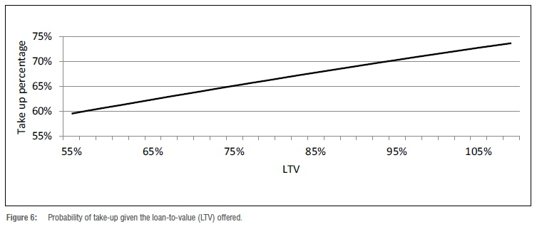
The Gini coefficient on the training data was 0.087 and on the validation data set was 0.093, with a 95% confidence interval of (0.084; 0.101). The Gini coefficient is much lower than the previous logistic regression developed for interest rates and we can reason that LTV has a much lower effect on take-up rates than does interest rate. Figure 6 illustrates the logistic regression equation fitted to LTV. We can see that the take-up rates now only vary between 59% and 74% (versus 0% to 90% in Figure 4).

Figure 6 shows the sensitivity of customers to LTV: the higher the LTV offered, the higher the take-up rate. This is not as prominent as the sensitivity of customers to interest rates when comparing Figure 4 with Figure 6. The reasoning behind this is that high-risk customers have limited options, as mentioned with interest rates. However, low-risk customers will either obtain a high LTV (resulting in take-up) or will be able to afford the deposit on a lower LTV loan (still resulting in take-up).

 

Predicting take-up rates using logistic regression

Now we consider the combination of variables in logistic regression. All available variables were tested using a stepwise regression and six of the variables were significant at a 0.1% p-value. We fitted a logistic regression equation (again using 5.5 years' of home loan data):

where

and where:

p is the probability of take-up;

X₁ is the recommended interest rate (interest rate offered to client);

X₂ is the LTV calculated by the LTV rules in place at that specific time;

X₃ is the Applicant Risk Grade;

X₄ is 1 or 0 for employment type;

X₅ is the type of loan; and

X₆ is 1 for new to home loans and 0 otherwise.

The Gini coefficient on the training data was 0.410 and on the validation data set was 0.403, with a 95% confidence interval of (0.396; 0.412). Using the absolute value of the standardised estimates, the importance of the six variables is as follows: 1. interest rate; 2. employment; 3. LTV; 4. new to home loan; 5. risk grade and 6. type of loan. The logistic regression with more variables increased the previous Gini coefficient (where only interest rate was used) from 0.314 to 0.403 -an improvement of 28% on the validation Gini coefficient. The increase in the Gini coefficient on the training data could be due to the fact that more variables were used.²⁸ The fact that the Gini coefficient on the validation data set is similar to that on the training data shows that our model is generalising well and will be able to predict new cases.²⁹ Logistic regression is a relatively simple technique, and the question arose whether a more complex technique could further improve the model performance.

 

Predicting take-up rates using tree-based ensemble models

We investigate two tree-based ensemble models: boosting and bagging. Other techniques were also investigated, such as neural networks, rule induction and support vector machines, but were found to be less effective. A brief explanation of each of these techniques and the related results are provided in the supplementary material.

All models were built using the SAS Enterprise Miner software. SAS is a statistical software suite developed by the SAS Institute for data management, advanced analytics, multivariate analysis, business intelligence, criminal investigation and predictive analytics.³⁰ SAS Enterprise Miner is an advanced analytics data mining tool intended to help users quickly develop descriptive and predictive models through a streamlined data mining process.³⁰

We have already mentioned that decision trees have several advantages and disadvantages and that ensemble models overcome these disadvantages while still maintaining the advantages. However, these ensemble models introduce their own disadvantages, namely the loss of interpretability and the transparency of model results. Bagging applies an unweighted resampling that uses random sampling with replacement, while boosting performs weighted resampling.

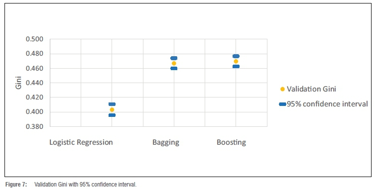
The bagging ensemble model resulted in a training Gini coefficient of 0.472 and a validation Gini coefficient of 0.467, with a 95% confidence interval of (0.460; 0.474). The boosting achieved similar results with a Gini coefficient on the training data set of 0.477 and on validation of 0.469, with a 95% confidence interval of (0.462; 0.477). From the Gini coefficient of 0.403 obtained previously using logistic regression, this improvement to 0.467 is a 16% increase on the validation Gini coefficient. The improvement of the Gini coefficient on the training data set could be due to the fact that we are using a more complex technique than logistic regression.²⁸ Note again the fact that the Gini coefficient on the validation data set is similar to the Gini coefficient on the training data, showing that the model did not overfit and in fact generalises well.²⁹

Figure 7 shows the validation Gini with the 95% confidence interval. The 16% improvement using bagging or boosting (tree-based ensemble) on Gini is clear, but this comes at a disadvantage: the loss of interpretability and transparency. An overall decision needs to be made whether the improvement outweighs the loss of interpretability.

A summary of the abovementioned modelling techniques considered in this paper is given in Table 1, including the Gini results of both the training and validation data sets. It is clear that the tree-based ensemble models (bagging and boosting) outperformed the logistic regression.

 

 

Further investigation

The customers who did not take up the home loan offer were further investigated to determine whether they subsequently took up another home loan at another institution. This was attempted by using bureau data. Unfortunately, only 13% of these non-take-ups were matched on the bureau as taking up another home loan at another institution. There are many reasons for the low match, including identification numbers not matching (this could be due to a joint account).

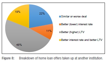
If the customers did take up another home loan, we investigated whether they took up a more attractive home loan offer in terms of interest rate and LTV. A higher LTV and a lower interest rate were considered better offers, and vice versa.

Figure 8 shows the breakdown of the home loans offered at another institution. The results indicate that 22% moved due to a similar or worse deal, 11% moved due to a better (i.e. lower) interest rate, 48% moved due to a better (i.e. higher) LTV, and 19% moved due to a better interest rate and a better LTV.

 

 

Conclusion and future research

The main contributions of this paper are threefold. Firstly, the effect of price elasticity in this specific South African's bank home loan database was illustrated. The higher the interest rate offered, the lower the take-up rate. Additionally, it was observed that high-risk customers are less sensitive to interest rate changes than are low-risk customers.

Secondly, we observed that home loan customers are sensitive to LTV: the higher the LTV offered, the higher the take-up rate (but not as sensitive as to interest rates offered). The 'chicken-and-egg' conundrum does pose some difficulty as the risk of a customer determines the LTV offered to the customer, and the LTV offered to the customer then influences the risk. Also, the LTV offered to the customer influences the take-up. A similar conundrum exists with interest rates.

Thirdly, models were built to predict the probability of take-up using home loan data over a 5.5-year period. Although logistic regression could predict take-up rates for home loan customers quite well, tree-based ensemble models can predict take-up rates more accurately (up to 16% improvement on validation Gini coefficients), but at a cost of interpretability.

The results of the bureau study indicate that 22% of customers moved to a home loan offered by another institution due to a similar or worse deal, 11% moved due to a better (i.e. lower) interest rate, 48% moved due to a better (i.e. higher) LTV, and 19% moved due to a better interest rate and a better LTV.

Many of the factors that influence take-up have not been captured into the models built in this paper, such as competitor offers, customer service, and so on. Unfortunately, it is very difficult to measure competitor offers. A future research topic could be to investigate the development of a factor that could reflect this influence.

With regard to adverse selection, lowering the interest rate could disproportionately draw high-risk customers.³¹ This paper once again confirms that choosing the appropriate interest rate for a home loan is not as straightforward as it may seem.⁴ In addition to general price sensitivity, adverse selection is an important characteristic in retail credit that is likely to have a significant impact on pricing.³² In related literature, various definitions of adverse selection can be found. For instance, there is a distinction made between adverse selection on observable information and adverse selection on hidden information.³³ Phillips and Raffard³⁴ make the same distinction but refer to direct and indirect adverse selection. A further research idea can be to investigate whether adverse selection exists in the South African home loan market. According to Thomas¹, adverse selection needs to be taken into account as part of risk-based pricing as it influences the interaction between the quality of the customers and the probability of them taking up credit products.

In this paper, the Gini coefficient was chosen to measure model lift. A future research investigation could be to add other measures and compare the results when using these measures.

Note that this paper addresses a subset of the main question: What is the optimal offer that a bank could make to a home loan client to ensure the maximum profit for the bank while still taking risk into account? To fully answer this question, all the underlying factors need to be identified, then understood and, if possible, used to model these factors. This paper started with the take-up probability, which is one of the factors influencing the main question. Future research could be to expand on this to address other factors that influence the answer to this question.

Another possible future research idea could be to investigate the effect of the LTV policy rules on the models built that contained LTV as a variable. This specific bank had certain LTV policy rules in place at specific times. These LTV rules were based on, among other criteria, property values and risk grades. For example, if the property value was less than ZAR1.5 million and the applicant risk grade was C, the maximum LTV allowed would be 85%. These LTV rules regularly change at the bank and the influence of these policy rules could be researched.

 

Acknowledgements

This work is based on research supported in part by the South African Department of Science and Innovation (DSI). The grantholder acknowledges that opinions, findings and conclusions or recommendations expressed in any publication generated by DSI-supported research are those of the author(s) and that the DSI accepts no liability whatsoever in this regard.

 

Competing interests

We declare that there are no competing interests.

 

Authors' contributions

T.V. was responsible for conceptualisation; methodology; data analysis; writing the initial draft; writing revisions and project leadership. S.H. and L.B. were responsible for conceptualisation; data collection; data analysis; writing revisions; and project management. B.B. was responsible for critical reading of the manuscript and suggesting revisions.

 

References

1. Thomas LC. Consumer credit models: Pricing, profit and portfolios. New York: Oxford University Press; 2009. http://dx.doi.org/10.1093/acprof:oso/9780199232130.001.1        [ Links ]

2. Otero-González L, Durán-Santomil P Lado-Sestayo R, Vivel-Búa M. The impact of loan-to-value on the default rate of residential mortgage-backed securities. J Credit Risk. 2016;12(3):1-13. http://dx.doi.org/10.21314/JCR.2016.210        [ Links ]

3. Phillips R. Pricing and revenue optimization. Stanford, CA: Stanford University Press; 2005.         [ Links ]

4. Huang B, Thomas LC. Credit card pricing and the impact of adverse selection. Discussion Papers in Centre for Risk Research. Southampton: University of Southampton; 2009.         [ Links ]

5. Terblanche SE, De la Rey T. Credit price optimisation within retail banking. Orion. 2014;30(2):85-102. http://dx.doi.org/10.5784/30-2-160        [ Links ]

6. Nagle T, Holden R. The strategy and tactics of pricing: A guide to profitable decision making. Upper Saddle River, NJ: Prentice Hall; 2002.         [ Links ]

7. Cross RG, Dixit A. Customer-centric pricing: The surprising secret for profitability. Bus Horiz. 2005;48:483-491. http://dx.doi.org/10.1016/j.bushor.2005.04.005        [ Links ]

8. Karlan DS, Zinman J. Credit elasticities in less-developed economies: Implications for microfinance. Am Econ Rev. 2008;98(3):1040-1068. http://dx.doi.org/10.1257/aer.98.3.1040        [ Links ]

9. Basel Committee on Banking Supervision. Basel II: International convergence of capital measurement and capital standards: A revised framework. Basel: Bank for International Settlements; 2006. Available from: https://www.bis.org/publ/bcbs128.pdf        [ Links ]

10. Basel Committee on Banking Supervision. High-level summary of Basel III reforms. Basel: Bank for International Settlements; 2017. Available from: https://www.bis.org/bcbs/publ/d424_hlsummary.pdf        [ Links ]

11. Engelman B, Rauhmeier R. The Basel II risk parameters: Estimation, validation, and stress testing. 2nd ed. Berlin: Springer; 2011.         [ Links ]

12. Breiman L. Bagging predictors. Mach Learn. 1996;24:123-140.         [ Links ]

13. Breiman L, Fredman J, Olsen R, Stone C. Classification and regression trees. Wadsworth, CA: Pacific Grove; 1984.         [ Links ]

14. Maldonado M, Dean J, Czika W, Haller S. Leveraging ensemble models in SAS Enterprise Miner. Paper SAS1332014. Cary, NC: SAS Institute Inc.; 2014. Available from: https://support.sas.com/resources/papers/proceedings14/SAS133-2014.pdf        [ Links ]

15. Schubert S. The power of the group processing facility in SAS Enterprise Miner. Paper SAS123-2010. Cary, NC: SAS Institute Inc.; 2010. Availabe from: https://support.sas.com/resources/papers/proceedings10/123-2010.pdf        [ Links ]

16. Tevet D. Exploring model lift: Is your model worth implementing? Actuarial Rev. 2013;40(2):10-13.         [ Links ]

17. Breed DG, Verster T. The benefits of segmentation: Evidence from a South African bank and other studies. S Afr J Sci. 2017;113(9/10), Art. #20160345. http://dx.doi.org/10.17159/sajs.2017/20160345        [ Links ]

18. Verster T. Autobin: A predictive approach towards automatic binning using data splitting. S Afr Statist J. 2018;52(2):139-155. https://hdl.handle.net/10520/EJC-10ca0d9e8d        [ Links ]

19. Anderson R. The credit scoring toolkit: Theory and practice for retail credit risk management and decision automation. New York: Oxford University Press; 2007.         [ Links ]

20. Siddiqi N. Credit risk scorecards. Hoboken, NJ: John Wiley & Sons; 2006.         [ Links ]

21. Property24. How banks assess loan applications [webpage on the internet]. c2011 [cited 2020 Feb 16]. Available from: https://www.property24.com/articles/how-banks-assess-loan-applications/14026        [ Links ]

22. Lightstone Property [homepage on the internet]. c2020 [cited 2020 Feb 16]. Available from: https://lightstoneproperty.co.za/RiskAssessmentServ.aspx        [ Links ]

23. Standard Bank. Home loans [webpage on the Internet]. c2020 [cited 2020 Feb 14]. Available from: https://www.standardbank.co.za/southafrica/personal/products-and-services/borrow-for-your-needs/home-loans/        [ Links ]

24. South African Reserve Bank [homepage on the Internet]. c2019 [cited 2020 Feb 15]. Available from: www.resbank.co.za/Research/Rates/Pages/Rates-Home.aspx        [ Links ]

25. Baesens B, Roesch D, Scheule H. Credit risk analytics: Measurement techniques, applications, and examples in SAS. Hoboken, NJ: Wiley; 2016.         [ Links ]

26. Picard R, Berk K. Data splitting. Am Stat. 1990;44(2):140-147. https://www.jstor.org/stable/2684155        [ Links ]

27. SAS Institute Inc. Applied analytics using SAS Enterprise Miner (SAS Institute course notes). Cary, NC: SAS Institute Inc.; 2015.         [ Links ]

28. Friedman J, Hastie T, Tibshirani R. The elements of statistical learning. Berlin: Springer; 2001. https://doi.org/10.1007/978-0-387-21606-5_14        [ Links ]

29. SAS Institute Inc. Predictive modelling using logistic regression (SAS Institute course notes). Cary, NC: SAS Institute Inc.; 2010.         [ Links ]

30. SAS Institute [homepage on the Internet]. c2020 [cited 2020 Feb 15]. Available from: www.sas.com        [ Links ]

31. Park S. Effects of price competition in the credit card industry. Econ Lett. 1997; 57:79-85. https://doi.org/10.1016/S0165-1765(97)81883-6        [ Links ]

32. Stiglitz J, Weiss A. Credit rationing in markets with imperfect information. Am Econ Rev. 1981;71(3):393-410. https://www.jstor.org/stable/1802787        [ Links ]

33. Ausubel LM. Adverse selection in the credit card market. c1999 [cited 2019 Jan 10]. Available from: http://www.ausubel.com/creditcard-papers/adverse.pdf        [ Links ]

34. Phillips RL, Raffard R. Theory and empirical evidence for price-driven adverse selection in consumer lending. Paper presented at: 4th Credit Scoring Conference; 2009 Aug 26-28; Edinburgh, Scotland.         [ Links ]

 

 

Correspondence:
Tanja Verster
Email: Tanja.Verster@nwu.ac.za

Received: 11 Nov. 2019
Revised: 05 May 2020
Accepted: 23 June 2020
Published: 29 Jan. 2021

 

 

Editor: Jane Carruthers
Funding: South African Department of Science and Innovation

 

 

Supplementary Data

The supplementary data is available in pdf: [Supplementary data]