RESEARCH ARTICLES

 

Estimating soil moisture using Sentinel-1 and Sentinel-2 sensors for dryland and palustrine wetland areas

 

 

Ridhwannah Gangat^I; Heidi van Deventer^{I, II}; Laven Naidoo^II; Elhadi Adam^I

^IArchaeology and Environmental Studies, Department of Geography, University of the Witwatersrand, Johannesburg, South Africa
^IICouncil for Scientific and Industrial Research, Pretoria, South Africa

Correspondence

 

 

---

ABSTRACT

Soil moisture content (SMC) plays an important role in the hydrological functioning of wetlands. Remote sensing shows potential for the quantification and monitoring of the SMC of palustrine wetlands; however, this technique remains to be assessed across a wetland-terrestrial gradient in South Africa. The ability of the Sentinel Synthetic Aperture Radar (SAR) and optical sensors, which are freely available from the European Space Agency, were evaluated to predict SMC for a palustrine wetland and surrounding terrestrial areas in the grassland biome of South Africa. The percentage of volumetric water content (%VWC) was measured across the wetland and terrestrial areas of the Colbyn Wetland Nature Reserve, located in the City of Tshwane Metropolitan Municipality of the Gauteng Province, using a handheld SMT-100 soil moisture meter at a depth of 5 cm during the peak and end of the hydroperiod in 2018. The %VWC was regressed against the Sentinel imagery, using random forest, simple linear and support vector machine regression models. Random forest yielded the highest prediction accuracies in comparison to the other models. The results indicate that the Sentinel images have the potential to be used to predict SMC with a high coefficient of determination (Sentinel-1 SAR = R²>0.9; Sentinel-2 optical = R²>٠.9) and a relatively low root mean square error (Sentinel-1 RMSE =<17%; Sentinel-2 optical = RMSE <21%). Predicted maps show higher ranges of SMC for wetlands (> 50%VWC; p<0.05) compared to terrestrial areas, and therefore SMC monitoring may benefit the inventorying of wetlands, as well as monitoring of their extent and ecological condition.
Significance: •The freely available and space-borne Sentinel sensors show potential for the quantification of surface soil moisture across a wetland-terrestrial gradient. •Significant differences between the surface soil moisture of palustrine wetlands and terrestrial areas, imply that inventorying and monitoring of the extent and hydroperiod of palustrine wetlands can potentially be done

Keywords: soil moisture content, volumetric water content, hydroperiod, random forest regression, machine learning regression models

---

 

 

Introduction

Globally, it is estimated that more than 85% of wetlands have been transformed, primarily owing to the loss of natural habitat resulting from land conversion, but also as a consequence of other pressures including changes to the hydrological regime, water pollution and invasive species.^1,2 In South Africa, the extent of natural and transformed wetlands is unknown^3,4, although sub-national studies have shown that 58% of wetlands in the Umfolozi secondary catchment (in the KwaZulu-Natal Province), had already been transformed irreversibly already by the 1990s⁵. Regional and automated inventorying and monitoring of wetland extent is critical for their conservation and management.

Remote sensing has played an important role in the detection and monitoring of the inundated sections of wetlands, both internationally and in South Africa. For example, the Global Inundation Extent from Multi-Satellites (GIEMS) and Global Surface Water Explorer products have been generated from coarse-scale satellite imagery which reflect the extent of inundation of larger artificial and natural wetlands.^6,7 In South Africa, the national land-cover products include open water classes^8, and, more recently, monitoring of the monthly extent of inundation⁹ has improved our ability to characterise the hydroperiod of wetlands. Yet early estimations of the extent of wetland cover showed that nearly 89% of wetlands are either arid or covered with vegetation (palustrine) in nature, whereas only 11% may be inundated.⁴ The development of indices which would characterise the extent and nature of palustrine wetlands is, therefore, a gap and top priority for South Africa.

Surface soil moisture is an important variable of palustrine wetlands that could potentially inform on the extent, hydroperiod and ecological condition of wetlands.¹⁰ Wetlands are areas where the soil becomes intermittently (±3 months in a year or less), seasonally (3-9 months per annum) or permanently (>9 months per annum) saturated within 50 cm from the soil surface.^11,12 Traditional in-situ methods to measure percentage volumetric water content (%VWC), which use the dielectric properties within the soil (for example, the gravimetric method), are limited in representing the spatial and temporal variations of soil moisture^13,14, and are also labour intensive, time consuming and costly¹⁵. Regional prediction of soil moisture content (SMC) through surface hydrological models has been stymied by the availability of coarse-scale data sets, in the range of ~10-100 km spatial resolution^16-19, which prohibits the prediction of SMC for the small wetland features of an arid to semi-arid country such as South Africa. As precipitation is highly variable across South Africa²⁰, frequent temporal updates of SMC would be essential to improve the understanding of soil saturation periods for wetlands. The prediction of SMC using space-borne sensors offers several advantages to traditional measurements and other modelling methods, the most important being that these sensors are able to estimate SMC frequently at regional scale.²¹

Several studies have investigated the capability of space-borne sensors (including both Synthetic Aperture Radar (SAR) and optical sensors) in estimating surface SMC (see review by Filion et al.²²). Some of the most recent studies done using the latest available sensor technology managed to achieve high coefficients of determination (R² = >0.72) and low root mean square errors (RMSEs <13%).^23-26 In general, the active SAR sensors were restricted to C-band sensors, which can penetrate between 5 cm and 10 cm into the canopy or soil, at a spatial resolution ranging from 10 m to 100 m. Passive L-band SAR sensors, on the other hand, can penetrate to a depth of 30 cm, and have spatial resolutions ranging from 3 km to 35 km²⁷; however, they are costly and not suitable for monitoring small wetlands. SAR sensors have the advantage over optical sensors in that they are not affected by cloud cover, yet scattering of the signal on highly textured areas and dense vegetation may reduce the accuracy of prediction. Optical sensors, in contrast to SAR sensors, cannot penetrate soil depth to estimate SMC, but infer SMC from the total reflectance of soil, vegetation and water across the visible/near infrared (VNIR: 400 nm-1200 nm) and the short-wave infrared (SWIR: 1200 nm-2500 nm) regions of the electromagnetic spectrum.²⁸ Unlike SAR sensors, detection of SMC using optical sensors is affected by cloud cover, cover texture and the density of vegetation.²⁹ The incorporation of vegetation indices, multiple phenological periods and different incident angles in the SMC predictions decreased the RMSE, and in this way, reduced the impact of vegetation on the prediction.^26,30,31 However, a study done by Hornacek et al.³² showed that vegetation ≤ 1 kg/m² had very little influence on the estimation of SMC in terrestrial systems. In general, critical limitations of these SAR and optical sensors for the estimation and monitoring of SMC are the spatial resolution of detection and cost. In an arid to semi-arid country such as South Africa, wetlands are small in extent, and palustrine wetlands often are composed of a mosaic of soil and vegetation cover. SMC therefore offers the advantage of a single variable to monitor across the landscape to inform wetland extent, hydroperiod and ecological condition.

The Sentinel SAR and optical sensors were launched between 2014 and 2017 by the European Space Agency (ESA) and consist of twin satellites each: Sentinel SAR Sentinel-1A and Sentinel-1B (S1A, S1B) and optical Sentinel-2A and Sentinel-2B (S2A, S2B). Images from these sensors were made freely available to the public and consequently offered several new opportunities for testing the capabilities of space-borne sensors in the quantification and monitoring of features on earth, including SMC of palustrine wetlands. These operational space-borne sensors hold promise for predicting SMC at a regional scale for palustrine wetlands in South Africa, but these sensors are yet to be assessed for their capabilities in the temperate regions of the southern hemisphere. In addition, none of the studies assessed SMC across a terrestrial-wetland gradient, and whether thresholds can be selected for determining the maximum extent of a wetland. Average %VWC values measured in terrestrial systems abroad ranged from 24% to 45%, while in-situ SMC measured in wetlands was generally approximately above 50%.^26,31,33

The aim of this study was therefore to determine whether the Sentinel-1 and Sentinel-2 sensors have potential to be used in estimating SMC across a gradient of palustrine wetlands to terrestrial areas in the grassland biome of South Africa. The grassland biome extends to approximately a third of the land mass of South Africa³⁴, hosts a number of palustrine wetlands, and is one of the biomes most threatened by multiple pressures such as land conversion to urban areas and mining³⁵. Our objectives were to (1) assess the capability of the SAR and optical Sentinel sensors in estimating SMC and (2) determine whether there are significant differences between SMC values between terrestrial areas and the wetlands, to inform a proposed threshold of wetland extent. We hope the outcome will contribute to South Africa's National Wetland Monitoring Programme.³⁶

 

Methods

Study area

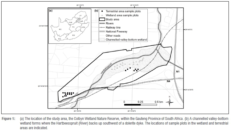
The study area (approximately 70 ha) was situated in the Colbyn Wetland Nature Reserve (CWNR), located in the City of Tshwane Metropolitan Municipality of the Gauteng Province, South Africa (25°44'21.67"S; 28°15'15.35"E) (Figure 1). The study area falls within the grassland biome and experiences a temperate climate with the rainfall season between September and March and the dry season between April and August. This ecoregion experiences an average summer rainfall of between 650 mm and 750 mm per annum and an evapotranspiration of 524 mm annually.³⁷

The Hartbeesspruit River drains the catchment, flowing in a northeasterly direction up to a dolerite dyke. The dolerite dyke forms a barrier on the northern side of the study area, and even though it has been breached by the river, water backs up southwest of the dyke, resulting in the formation of a channelled valley-bottom wetland. The adjacent hillside slopes contribute seepage towards the wetland, and groundwater also contributes interflow towards the channel.³⁸ Most of the wetland remains permanently saturated throughout the year, and peat has been found in the centre part of the wetland near the channel (extent estimated at 4.68 ha).³⁹ The CWNR is considered a palustrine wetland, with the full cover of grasses and sedges dominating in the temporary saturated zones of the wetland (e.g. cotton wool grass or Imperata cylindrica) and reeds (Phragmites australis), bulrush (Typha capensis) and the lesser pond sedge (Carex acutiformis) in the permanently saturated zones.⁴⁰ Only the river channel has open water partly visible on satellite imagery, lined by exotic tree species, such as the weeping willow (Salix babylonica) and poplars (Populus × canescense), with the latter also found in a part of the permanently saturated zone of the wetland.

The CWNR is exposed to a number of pressures and impacts. Drainage has been disrupted by numerous roads, resulting in high energy run-off leading to erosion of the wetland.⁴¹ Weirs have been built along the channel to alleviate the effects of erosion in order to prevent further degradation of the wetland.⁴² The Koedoespoort Railway line crosses through the CWNR, causing soil compaction which results in an increase in soil moisture saturation in parts of the study area.

 

Data collection

Image acquisition and pre-processing

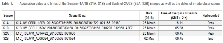
Sentinel-1 SAR data acquisition and pre-processing

The S1A and S1B SAR C-band images were downloaded as Ground Range Detected (GRD) data (10x10 m spatial resolution) from the Copernicus website (https://scihub.copernicus.eu/dhus/#/home) (Table 1). The data were acquired in Interferometric Wide (IW) for both the vertical-transmit, vertical-receive (VV) and vertical-transmit, horizontal-receive (VH) polarisation modes. S1A and S1B GRD data were pre-processed using ESA's Sentinel Application Platform (SNAP) software version 6.0 (2018) for radiometric calibration, multi-looking and terrain correction. Multi-looking was applied to each Sentinel-1 image (applying 2 and 2 multi-looking factors for range and azimuth, respectively) to reduce the speckle present in the images which subsequently converts the 10-m spatial resolution image to a 20-m spatial resolution image. Radiometric calibration of the SAR images converts the data from a digital number format to backscatter in sigma naught or sigma dB. Backscatter signal errors associated with terrain, orientation and geo-referencing of the imagery were corrected with the Range Doppler Terrain Correction using the Shuttle Radar Topography Mission 3 arc-seconds 30-m digital elevation model.⁴³

Sentinel-2 data acquisition and pre-processing

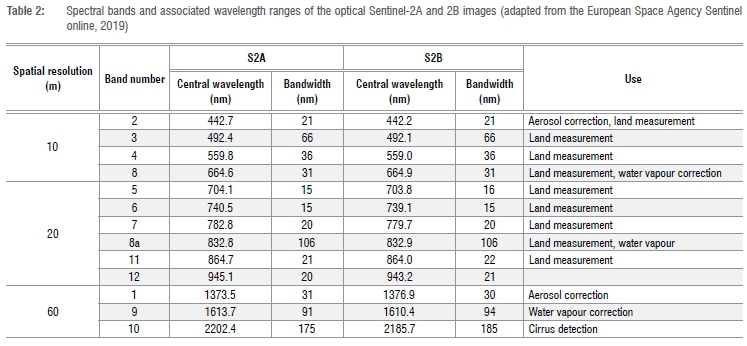
Sentinel-2 optical images (S2A and S2B), processed to Level 1C, were acquired as close as possible to the SAR images, but avoiding imagery with >20% cloud coverage (Table 1). The images were downloaded from the United States Geological Survey (USGS) Earth Explorer website⁴⁴ as 10 individual spectral bands (Table 2). Bands 2, 3, 4 and 8 are provided by ESA at a 10-m spatial resolution while bands 5, 6, 7, 8a, 11 and 12 are at 20-m spatial resolution. Bands with a 60-m spatial resolution (bands 1, 9 and 10) are mainly used in atmospheric correction and cirrus-cloud screening and were not required for estimating the percentage SMC (%SMC). Three procedures were necessary for pre-processing the Sentinel-2 satellite images: (1) atmospheric correction; (2) resampling the 20-m multispectral images to 10 m using the Sen2Cor algorithm using the default settings in SNAP; and (3) sub-setting to extract the study area.

In-situ soil moisture collection

Prior to sampling, several field visits were made to plan sampling positions in the wetland and terrestrial areas. The extent of the wetland was guided by the National Wetlands Map 5⁴, and identified through characterising the nature of the soil, extracted from the ground using a soil auger, as well as vegetation species as indicator plants. Subsequent to this first scoping field visit, the boundaries of the channelled valley-bottom wetland were adjusted to match field observations of terrestrial and wetland areas, resulting in an extent of 28.7 ha (Figure 1). The sampling period was selected to coincide with the peak hydroperiod, which would help to detect the maximum level and extent of soil moisture in the wetland for wetland inventorying. A stratified random sampling method was chosen to collect in-situ, %VWC measurements in the wetland and terrestrial areas. Stratified random sampling ensured that the point sample measurements were well distributed in order to represent the wetland and terrestrial sampling areas. Available Sentinel images were downloaded and used to determine suitable positions for the sampling plots which were positioned to fit both the Sentinel SAR and optical image pixels. A sampling plot the size of 10 m x 10 m was positioned within a 20 m x 20 m pixel of the Sentinel-1 and Sentinel-2 image pixels. A total of 40 sampling plots was planned for the field survey, with 20 located in the wetland area and 20 located in the terrestrial area (Figure 1). For each sample plot, five replicate measurements of %VWC were recorded in order to capture the variation of the observed %SMC within the top layer of the soil surface. This yielded a total of 200 readings for the terrestrial and wetland areas during each sampling campaign.

Near-surface volumetric SMC was acquired using a handheld SMT-100 soil moisture and temperature probe.⁴⁵ The probe measures the %VWC at a depth of 5 cm. The centre and corners of each sample plot were mapped in ArcGIS version 10.5⁴⁶ and then uploaded to several e-Trex 30 Global Positioning System (GPS) devices.⁴⁷ The GPS devices were then used to navigate to the same location for successive sampling campaigns. Previous studies recommended that ground measurements should be made within a 2-h window period around the sensor overpass time so as to minimise diurnal variation in SMC and vegetation on radar backscatter.^48,49 Therefore, three probes were used by three teams to record the %VWC within a 2-h time period around the satellite overpass, which included the hour before and after the time of overpass of each Sentinel sensor.

To determine the impact of vegetation on the regression, the vegetation height in various zones was randomly measured and recorded during the field campaigns. In general, the density and height of the vegetation in both zones varied little for the duration of %VWC data collection between March and May of 2018. Regardless, sample plots were planned at least 2 m away from macrophytes and trees where the height of the vegetation was >2 m high. In general, the canopy height in sample plots of similar grassland palustrine wetland sites (Chrissiesmeer, Mpumalanga Province) was 1.5-2 m, with an estimated biomass ≤850 g/m².⁵⁰ The Normalised Difference Vegetation Index (NDVI)^51,52 is often used to compensate for the influence of vegetation in estimating SMC^24,49. However, according to Hornacek et al.³², vegetation and texture have very little impact on the %SMC modelling if grass vegetation is ≤1 kg/m². Consequently, no adjustments were made for vegetation in this paper, because the above-ground biomass and sedges in the study area are likely <850 g/m².

Data analysis

In order to assess the Sentinel sensors' capability to estimate the SMC, backscatter from S1A and S1B and reflectance values from S2A and S2B were extracted from the respective images and regressed against the average of the five in-situ %VWC measurements taken for each plot. The centre point recorded for each sample plot in shapefile format was used to extract backscatter values for VV, VH polarisation modes as well as VV+VH as a modelling scenario, in ArcMap 10.5.⁴⁶ Similarly, the spectral reflectance values of the optical sensors were extracted for all the bands, excluding bands 1, 9 and 10 (60-m resolution bands) for the same points.

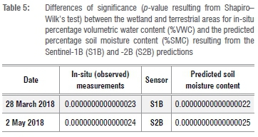
The Sentinel-1 backscatter values and Sentinel-2 reflectance band values were regressed against the %VWC values (in-situ measurements) using both a parametric (the simple linear regression model or SLR) and two non-parametric (support vector machine - SVM and random forest - RF) algorithms in the Waikato Environment for Knowledge Analysis (Weka) software version 3.8.⁵³ These regression models are commonly used in the remote sensing of environmental variables and the capabilities of these models were compared in this study (see review by Gangat²⁶). In principal, parametric models assume normal distribution of the data, and hence they depend on mean and standard deviation statistics. These models are less complex in terms of tuning and require a fixed number of input variables.⁵⁴ Non-parametric models do not assume normal distribution and, as spectral data are often not normally distributed, non-parametric methods have been found to outperform parametric methods in remote sensing classification and prediction. A data split was used with 30% data for the training data set and 70% for the validation data set to test the best model for regressing the observed %VWC to the estimated %SMC. Individual polarisations and bands as well as a combination of the polarisations and all bands were evaluated for each sensor in predicting %SMC. The best model to predict %SMC from the radar and optical images was selected where the highest coefficient of determination (R²) and lowest RMSE was attained. In order to estimate the %SMC, backscatter from S1B and reflectance values from optical S2B were extracted from the respective images. A Shapiro-Wilk test was used to test the differences between the wetland and terrestrial areas, for both the in-situ %VWC and predicted %SMC, to assess whether thresholding would be possible for wetland mapping. A p<0.05 was used to identify significant differences.

 

Results

Ability of Sentinel-1 and Sentinel-2 to estimate soil moisture content

Of the various modelling scenarios, the Sentinel images were capable of predicting the %SMC with the majority of coefficients of determination (R²)>0.7 and RMSEs<21% (Table 3). Of the four sensors which used RF, S1B produced a high R² of 0.92-0.94 and the lowest RMSE of 10%. S2B achieved the second-highest results with an R² of 0.92-0.94 and RMSE of 12-14%. S2A produced slightly better results (R =0.70-0.86; RMSE=13-20%) than S1A, which resulted in the lowest R² of 0.58-0.72 and highest error at RMSE=19-24%.

 

 

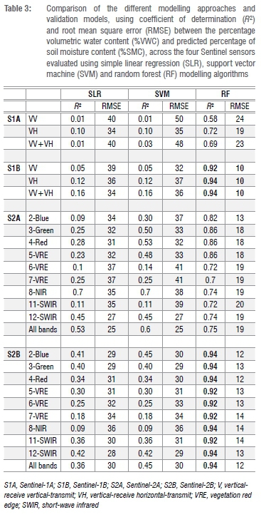
Of the three polarisation modes (VV, VH and VH+VV) associated with the two Sentinel-1 (SAR) sensors, the VH polarisation mode and the VH+VV modelling scenario yielded higher accuracies (R²>0.7) and lower errors (RMSE<19%) than the VV polarisation (Table 3). S1B showed the highest coefficient of determination (R²>0.9) when the VH polarisation and VH+VV modelling scenario were used, with an RMSE of 10% in both instances. The results for S1A were slightly lower at R²=0.72, with a slightly higher RMSE of 19% for VH and 23% for VH+VV. The single VV polarisation showed the lowest coefficient of determination and highest error (R²=>0.58; RMSE = >24%) for both of the Sentinel-1 sensors where the RF algorithm was used. The VH polarisation mode, however, contributed more to the accuracies of the combined VH+VV modelling scenario inputs than the single polarisation (VV) mode.

A combination of all the bands for the optical sensors S2A and S2B, in general, resulted in high accuracies (R²>0.7 and RMSE<20%) when the RF algorithm was used, whereas the SLR and SVM showed an R²<٠.٦ and RMSE were 30-50% (Table 3). Some exceptions are evident where the use of the blue, green, red and vegetation red edge (VRE) bands produced comparable results to the combined bands, most noticeably when the RF algorithm was used (R²=0.7 for S2A, or even higher for S2B (R²>0.9). Five of the S2B individual bands resulted in the highest coefficients of determination in predicting %SMC (R²=>0.94; RMSE=13%), namely: blue (band 2:496-492 nm), green (band 3: 560-559 nm), red (band 4: 664-665 nm), NIR (band 8: 833-835 nm) and SWIR (band 12: 2185-2204 nm).

When comparing the regression model scenarios, the RF algorithm outperformed the SLR and SVM. RF achieved ranges of the coefficients of determination from R²=٠.٥٨ to R²=٠.٩٤ and RMSE values between ١٠٪ and ٢٤٪ (Table 3). In contrast, the non-parametric SVM had lower accuracies ranging from R²=٠.٠١ to R²=٠.7 and RMSE values between 25% and 50%. The parametric SLR algorithm showed similar ranges of coefficients of determination to that of the non-parametric SVM algorithm (from R² = 0.01 to R² = ٠.7) and RMSE values ranging from 25% to 40%. Consequently, the RF algorithm was applied to the S1B SAR, using only VH polarisation which contributed most to the backscatter values, and all the bands from the S2B image, to predict %SMC for the CWNR.

Comparison of observed %VWC and predicted %SMC in wetland and terrestrial areas

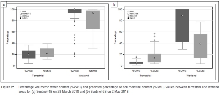
In-situ observed %VWC ranged from 16% to 100% in the wetland areas and from 1% to 37% for the terrestrial area (Table 4). In comparison, the S1B predicted %SMC ranged from 30% to 100% for wetlands and 11% to 39% for terrestrial areas, and the S2B predicted %SMC ranged from 4% to 78% in the wetlands and 4% to 57% in the terrestrial areas. The mean soil moisture values for in-situ observed %VWC in the wetlands and terrestrial areas were higher on 28 March 2018 (mean±standard deviation = ٩1%±٢١ and 20%±٨, respectively) compared to those measured a month later on 2 May 2018 (mean±standard deviation = 74%±٢٧ and 6%±٣, respectively). Similar trends were visible in the predicted %SMC mean values for both the wetland and terrestrial areas. In contrast, the percentage of coefficient of variance (%COV) showed an increase over the month (from 28 March 2018 to 2 May 2018), for both the in-situ %VWC and %SMC predicted from both sensors, within the wetland and terrestrial areas. In general, the %COV was much lower in the terrestrial area for both dates, considering the %VWC and %SMC, compared to the wetland area (Figure 2).

 

 

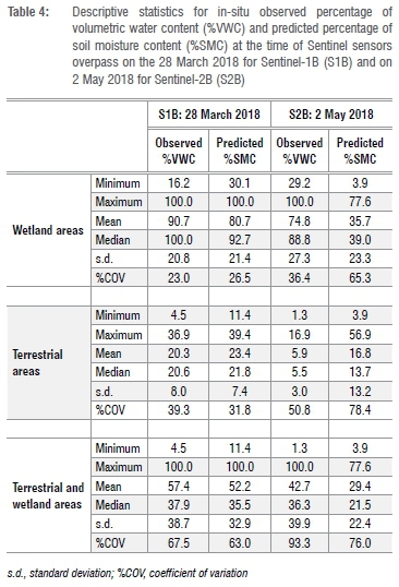
Soil moisture values, whether in-situ %VWC or predicted %SMC, were significantly different between the wetland and terrestrial areas for both dates (Table 5). The overlap in the minimum %VWC and %SMC with the maximum %VWC and %SMC (Table 4) showed that there is still confusion in the soil moisture values between the wetland and terrestrial areas, which makes it difficult to identify a certain threshold for wetland mapping. An average threshold of 50%VWC and/or 50%SMC was therefore used to distinguish wetland extent from the terrestrial areas.

 

 

Predicted soil moisture maps for the study area

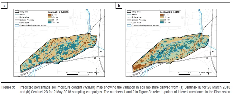
The predicted %SMC maps from the S1B and S2B sensors show a variation in the extent of soil saturation (Figure 3a and 3b). Although differences are visible between the S1B and S2B predictions on the edges of the study area, both maps show a higher level of soil saturation in the centre of the channelled valley-bottom wetland, southeast of the Hartbeesspruit River's channel. These areas read nearly 100% of %VWC during the sampling for both dates.

Using the 50% threshold, nearly 47% (32.7 ha) of the extent of the study area could be wetland from the S1B prediction (Figure 3a), whereas approximately 23% (15.7 ha) would be predicted as wetland when using the S2B %SMC map (Figure 3b).

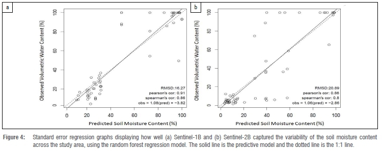
The standard error graphs illustrating the observed in-situ %VWC against the predicted %SMC, represent the level of overestimation and underestimation of the model (Figure 4a and 4b). The results displayed show a coefficient of determination for S1B of R²=0.91 and for S2B of R²=0.86. Both S1B and S2B showed that observed %VWC values of under 50% are expected to be underpredicted, whereas above this threshold, predicted %SMC is overestimated, in each case by 16% and 21%, respectively (Figure 4).

 

Discussion

This study showed that the freely available Sentinel SAR and optical sensor data have potential for estimating soil moisture in palustrine wetlands. These sensors were used to predict SMC for a palustrine wetland in the grassland biome of South Africa with a RF algorithm resulting in a high coefficient of determination (R²=>0.7) and a low RMSE= <24% using various modelling scenarios. The results are comparable to those of other studies done within wetland and terrestrial areas in temperate climates of Poland, Germany and Italy.^23-26 Further work is required to test the capabilities of these Sentinel sensors across other palustrine wetlands in South Africa, to assess the potential for upscaling the sensors for wetland inventorying and monitoring.

Soil moisture ranges showed significant differences between the wetland and terrestrial areas. Although the wetland-terrestrial gradient and a threshold for wetland mapping have not been explored in other studies, their measured SMC values were compared to this study to assess such a threshold. In Germany, the %VWC was 30-99.1%VWC with a mean of 50%VWC over a floodplain with a grass canopy of up to 2 m in height, measured at the end of the growth period.²⁶ In Italy, the mean %VWC in a dense terrestrial grassland area was 45%VWC at the end of the growth period.³¹ A study conducted on the coastal plains of Washington District Capital (USA) attained an average of 59%VWC for their wetland areas and 24%VWC in the terrestrial areas.³³ Our findings show mean soil moisture levels for the in-situ measured data in the wetland of >75%VWC - significantly higher (p<0.05) compared to the mean %VWC measured in the terrestrial area (20% and 6% on the 28 March and 2 May 2018, respectively). An overlap in %VWC and %SMC values still makes it difficult to identify a threshold for mapped wetlands with high confidence. Consequently, we propose an interim 50% threshold for measured %VWC or predicted %SMC to distinguish the extent of the wetland in the CWNR for these two dates. Continuous assessment of the different soil moisture ranges over multiple time periods and hydrological regimes would be critical to confirm this proposed threshold and would provide insight into determining the maximum extent of wetlands.

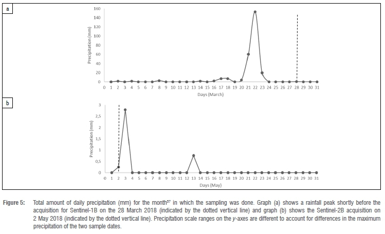
The site showed a variation in the magnitude and areal extent of soil moisture between 28 March 2018 and 2 May 2018. The magnitude of the mean observed %VWC decreased from 28 March to 2 May by 6%. The predicted %SMC also showed a decline - by 45% - which may be explained by differences in prediction of %SMC by the radar and optical sensors. Regardless, it appears as if the sensors would have the potential to detect the variation in the degree of soil saturation. The predicted %SMC maps of 28 March 2018 (using S1B) and 2 May 2018 (using S2B) showed differences in the areal extent of soil saturation across the wetland, which could be attributed to a variation in rainfall and the subsequent infiltration and interflow of water into the soil. If a 50%SMC threshold is used to extract the areal extent of the wetland, the extent of the wetland covered 47% or 32.7 ha on 28 March and 23% or 15.7 ha on 2 May. Interestingly, the sampling campaign on 28 March 2018 took place shortly after an intense rainfall storm (22 March 2018) whereas the sampling campaign on 2 May 2018 took place approximately 2 weeks after a less intense rainfall period (Figure 5). This could possibly explain the higher mean values of 91%VWC and 23%COV recorded directly after the rain spell within the top layer of the soil, which subsequently may have infiltrated to deeper soils a month later, resulting in a lower mean of 75%VWC and 6%COV. Theoretically, the continuous rainfall events over summer (rainfall started approximately mid-February of 2018)³⁷ would lead to progressively accumulated water in the main part of the channelled valley-bottom wetland through surface run-off and groundwater accumulation. The accumulation of water in soil of the palustrine wetland would have resulted in an increase in the dielectric constant, resulting in higher backscatter and reflectance values. These results are evident from the comparison between the predicted SMC maps from S1B and S2B, which suggests that changes in soil saturation could potentially be used to detect soil saturation across a wetland's hydroperiod. We recommend that both sensors be used to test whether a more refined threshold for wetland mapping can be derived from time-series data.

In modelling SMC with the use of satellite imagery, our methods show that the RF non-parametric algorithm outperformed the SLR and SVM algorithms. This finding is in line with other studies in which non-parametric algorithms outperformed parametric algorithms.^54,55 Our study showed a minor difference in model performance for the radar data when using either VV, VH or VV+VH polarisation (R²>0.92 and RMSE=10%). This differs from the findings of Dabrowska-Zielinska et al.²⁴, who indicated that the SAR VH outperforms VV and dual polarisation. For the optical data, the use of all bands achieved the highest R² (0.94) and the lowest RMSE (12%), compared to the use of individual bands. The use of bands across the visible, NIR and SWIR all contributed to the optimisation of the prediction of %SMC in the RF algorithm.

When comparing the parametric and non-parametric predictive models (SLR, RF and SVM), the comparative evaluation results show that RF outperformed the other parametric SLR and non-parametric SVM. RF resulted in the highest coefficients of determination (R² ٠.٧-0.94) when either VV+VH or all optical bands were used. In contrast, the SLR and SVM show a poorer relationship between %VWC and %SMC when all bands were used (R² ranged from ٠.٤-0.6), while for the radar, SLR showed no relation (R²<٠.٢). In general, non-parametric models are more suitable for reflectance and backscatter data, because these are often not normally distributed.^50,55 In addition, the non-parametric models are able to predict values using data sets with fewer observations over large regions. Although RF and SVM often show comparative results in remote sensing prediction of continuous variables, SVM requires more customisation to obtain the optimum model performance, whereas RF is easier to use and does not require reiterative testing.

Despite the concern of the influence of vegetation on backscatter or reflectance data, our results show that it was likely not a significant influence on the prediction of %SMC in the case of CWNR. Above-ground biomass values for palustrine wetlands in the grassland biome of South Africa are estimated to be <850 g/m²⁽⁵⁰⁾ and <1 kg/m²⁽³²⁾, and are considered to have very little influence on the estimation of SMC. The inclusion of NDVI in the S2B regression showed a minor increase in model performance (R²=٠.٩ and RMSE of ٠.٢; results not shown). Further work is required to assess whether vegetation and texture indices improve the estimation of SMC in other sites and climatic regions.

Regional monitoring of soil moisture would contribute greatly to South Africa's National Wetland Monitoring Programme, particularly because it is a common variable across palustrine wetland type, whereas vegetation communities would vary. To date, the SAR sensors available for the estimation of SMC are limited to C-band sensors, which can penetrate only to a depth of 5 cm. L-band sensors, on the other hand, have the advantage of deeper penetration through canopy cover or into bare soils. The Advanced Land Observing Satellite (ALOS)-2 L-band SAR sensor of the Japan Aerospace Exploration Agency (JAXA) has a high spatial resolution (10 m) and a temporal resolution of 46 days; however, these data were not freely available for use in monitoring at the time of this study, but the Japanese ministry announced in November 2019 that the ALOS archive would be made openly accessible. Several L-band sensors are planned to be launched from 2020 onwards, potentially for public use, including ALOS-3 from JAXA, NASA ISRO Synthetic Aperture Radar (NISAR) from NASA/ISRO and TanDEM-L from the German Space Agency.⁵⁶

 

Conclusion

This study proves that the freely available Sentinel-1 (SAR) and Sentinel-2 (optical) sensors have potential in the estimation of the extent and degree of soil saturation in palustrine wetlands in the grassland biome of South Africa. The Sentinel-1 SAR and Sentinel-2 optical sensors were able to predict %SMC with a high coefficient of determination (R²>٠.9) and low RMSE (<21%) along a wetland-terrestrial gradient in the grassland biome of the Gauteng Province of South Africa. The non-parametric RF algorithm outperformed the parametric SLR and non-parametric SVM algorithms in predicting %SMC for the CWNR during the peak of the hydroperiod in March and May 2018. Significant differences between the surface soil moisture of the palustrine wetland and the surrounding terrestrial areas imply that inventorying and monitoring of the extent and hydroperiod of palustrine wetlands can potentially be done. An SMC threshold of ≥50% was used as a potential threshold to determine the extent of the wetland area; however, owing to uncertainties resulting from the overlap in the measured %VWC, further work would be required to confirm whether this threshold is relevant across the hydroperiod and other grassland sites. The predictions for the two months (March and May) showed a potential accumulation of soil saturation over the period, which may have resulted from interflow and groundwater accumulation. Although other studies suggest that vegetation has an influence on the prediction of soil moisture over an area, the incorporation of the NDVI in predicting %SMC from the optical Sentinel-2B image, showed only a minor improvement in the prediction. The prediction of SMC in the grassland biome of South Africa can play a significant role in improving the representation of the natural variation in soil saturation values of palustrine wetlands and enables the detection of outlier seasons or years associated with the impacts of global and changing climate.

 

Acknowledgements

This work was funded by the South African Water Research Commission (WRC) under the project K5/2545 'Establishing remote sensing toolkits for monitoring freshwater ecosystems under global change' as well as the Council for Scientific and Industrial Research (CSIR) through the project titled 'Common Multi-Domain Development Platform (CMDP) to Realise National Value of the Sentinel sensors for various land, freshwater and marine societal benefit areas'. Several fieldwork assistants have kindly contributed time, including Razeen Gangat, Mohamed Gangat, Taskeen Gangat, Zahra Varachia, Salman Mia, Yonwaba Atyosi and Jason le Roux. A special thanks to Tamsyn Sherwill from the WRC for including us in some of the Colbyn Wetland Nature Reserve projects and conservation initiatives.

 

Authors' contributions

R.G.: Student who undertook the literature search, planned the fieldwork, coordinated the fieldwork, did the analysis, and drafted the research output. H.v.D.: Primary supervisor who provided guidance to the student on the formulation of the research question, hypothesis, and execution of the fieldwork, participated in the fieldwork, and revised and edited the research output. L.N.: Co-supervisor who provided guidance to the student on the execution of the fieldwork, participated in the fieldwork, analysed the radar data and provided input and edits to the draft and revised research output. E.A.: Co-supervisor who provided a review of the research output.

 

References

1.Dudgeon D, Arthington AH, Gessner MO, Kawabata ZI, Knowler DJ, Lévêque C, et al. Freshwater biodiversity: Importance, threats, status and conservation challenges. Biol Rev. 2006;81(2):163-182. https://doi.org/10.1017/S1464793105006950        [ Links ]

2.Díaz S, Settele J, Brondízio E, Ngo HT, Guèze M, Agard J, et al. Summary for policymakers of the global assessment report on biodiversity and ecosystem services of the Intergovernmental Science-Policy Platform on Biodiversity and Ecosystem Services [document on the Internet].         [ Links ] c2019 [cited 2020 Mar 13]. Available from: https://www.ipbes.net/sites/default/files/downloads/spm_unedited_advance_for_posting_htn.pdf

3.Van Deventer H, Smith-Adao L, Mbona N, Petersen C, Skowno A, Collins NB, et al. South African Inventory of Inland Aquatic Ecosystems (SAIIAE). Report number CSIR/NRE/ECOS/IR/2018/0001/A. Pretoria: South African National Biodiversity Institute; 2018. http://hdl.handle.net/20.500.12143/5847        [ Links ]

4.Van Deventer H, Van Niekerk L, Adams J, Dinala MK, Gangat R, Lamberth SJ, et al. National Wetland Map 5 - An improved spatial extent and representation of inland aquatic and estuarine ecosystems in South Africa. Water SA. 2020;46(1):66-79. https://doi.org/10.17159/wsa/2020.v46.i1.7887        [ Links ]

5.Begg GW. The wetlands of Natal (Part 2): The distribution, extent and status of wetlands in the Mfolozi catchment. Report 71. Pietermaritzburg: Natal Town and Regional Planning Commission; 1988.         [ Links ]

6.Fluet-Chouinard E, Lehner B, Rebelo LM, Papa F, Hamilton SK. Development of a global inundation map at high spatial resolution from topographic downscaling of coarse-scale remote sensing data. Remote Sens Environ. 2015;158:348-361. http://dx.doi.org/10.1016/j.rse.2014.10.015        [ Links ]

7.Pekel J-F, Cottam A, Gorelick N, Belward AS. High-resolution mapping of global surface water and its long-term changes. Nature. 2016;540:418-422. https://doi.org/10.1038/nature20584        [ Links ]

8.GeoTerraImage (GTI). Technical report 2013/2014: South African national land cover dataset version 5. Pretoria: GTI; 2015.         [ Links ]

9.Thompson M, Hiestermann J, Moyo L, Mpe T. Cloud-based monitoring of SA's water resources. Position IT Magazine. 2018;38-41.         [ Links ]

10.Erwin KL. Wetlands and global climate change: The role of wetland restoration in a changing world. Wetl Ecol Manag. 2008;17:71-84. https://doi.org/10.1007/s11273-008-9119-1        [ Links ]

11.Burton TM, Tiner RW. Ecology of wetlands. In: Gene E, Likens GE, editors. Encyclopedia of inland waters. Oxford: Academic Press; 2009. p. 507-515. https://doi.org/10.1016/B978-012370626-3.00056-9        [ Links ]

12.Ollis D, Snaddon K, Job N, Mbona N. Classification system for wetlands and other aquatic ecosystems in South Africa: User manual: Inland systems. SANBI Biodiversity Series 22. Pretoria: South African National Biodiversity Institute; 2013.         [ Links ]

13.Engman ET. Applications of microwave remote-sensing of soil-moisture for water-resources and agriculture. Remote Sens Environ. 1991;35:213-226. https://doi.org/10.1016/0034-4257(91)90013-V        [ Links ]

14.Wood EF, Lettenmaier DP, Zartarian VG. A landsurface hydrology parameterization with subgrid variability for general circulation models. J Geophys Res. 1992;97:2717-2728. https://doi.org/10.1029/91JD01786        [ Links ]

15.Santi E, Paloscia S, Pettinato S, Notarnicola C, Pasolli L, Pistocchi A. Comparison between SAR soil moisture estimates and hydrological model simulations over the Scrivia Test Site. Remote Sens. 2013;5(10):4961-4976. https://doi.org/10.3390/rs5104961        [ Links ]

16.McDonnell JJ, Sivapalan M, Vaché K, Dunn S, Grant G, Haggerty R, et al. Moving beyond heterogeneity and process complexity: A new vision for watershed hydrology. Water Resour Res. 2007;43, W07301. https://doi.org/10.1029/2006WR005467        [ Links ]

17.Crow WT, Yilmaz MT. The Auto-Tuned Land Assimilation System (ATLAS). Water Resour Res. 2014;50:371-385. https://doi.org/10.1002/2013WR014550        [ Links ]

18.Riley W, Shen C. Characterizing coarse-resolution watershed soil moisture heterogeneity using fine-scale simulations. Hydrol Earth Syst Sci. 2014;18:2463-2483. https://doi.org/10.5194/hess-18-2463-2014        [ Links ]

19.Tebbs E, Gerard F, Petrie A, De Witte E. Emerging and potential future applications of satellite-based soil moisture products. In: Petropoulos GP, Srivastava P, Kerr Y, editors. Satellite soil moisture retrieval: Techniques and applications. Amsterdam: Elsevier; 2016; p. 379-400. https://doi.org/10.1016/B978-0-12-803388-3.00019-X        [ Links ]

20.Schulze RE, Lynch SD. Annual precipitation. In: Schulze RE, editor. South African atlas of climatology and agrohydrology. WRC Report no. 1489/1/06, Section 6.2. Pretoria: Water Research Commission; 2007.         [ Links ]

21.Wang L, Qu J. Satellite remote sensing applications for surface soil moisture monitoring: A review. Fron Earth Sci. 2009;3(2):237-247. https://doi.org/10.1007/s11707-009-0023-7        [ Links ]

22.Filion R, Bernier M, Paniconi C, Chokmani K, Melis M, Soddu A, et al. Remote sensing for mapping soil moisture and drainage potential in semi-arid regions: Applications to the Campidano plain of Sardinia, Italy. Sci Total Environ. 2015;543:862-876. https://doi.org/10.1016/j.scitotenv.2015.07.068        [ Links ]

23.Sadeghi M, Babaeian E, Tuller M, Jones S. The optical trapezoid model: A novel approach to remote sensing of soil moisture applied to Sentinel-2 and Landsat-8 observations. Remote Sens Environ. 2017;198:52-68. https://doi.org/10.1016/j.rse.2017.05.041        [ Links ]

24.Dabrowska-Zielinska K, Musial J, Malinska A, Budzynska M, Gurdak R, Kiryla W, et al. Soil moisture in the Biebrza Wetlands retrieved from Sentinel-1 imagery. Remote Sens. 2018;10:1979. https://doi.org/10.3390/rs10121979        [ Links ]

25.Holtgrave A, Forster M, Greifeneder F, Notarnicola C, Kleinschmit B. Estimation of soil moisture in vegetation-covered floodplains with Sentinel-1 SAR using support vector regression. Photogramm Eng Remote Sensing. 2018;86:85-101. https://doi.org/10.1007/s41064-018-0045-4        [ Links ]

26.Gangat R. Assessing whether soil moisture content (SMC) can be estimated for wetlands in the grassland biome of South Africa using freely available space-borne sensors [MSc thesis]. Johannesburg: University of the Witwatersrand; 2019.         [ Links ]

27. Klinke R, Kuechly H, Frick A, Förster M, Schmidt T, Holtgrave A, et al. Indicator-based soil moisture monitoring of wetlands by utilizing Sentinel and Landsat remote sensing data. Photogramm Eng Remote Sensing. 2018;86(2):71-84. https://doi.org/10.1007/s41064-018-0044-5        [ Links ]

28.Lu N, Chen S, Wilske B, Sun G, Chen J. Evapotranspiration and soil water relationships in a range of disturbed and understood ecosystems in the semi-arid Inner Mongolia, China. J Plant Ecol. 2001;4(1-2):49-60. https://doi.org/10.1093/jpe/rtq035        [ Links ]

29.Saalovaara K, Thessler S, Malik RN, Tuomisto H. Classification of Amazonian primary rain forest vegetation using Landsat ETM+ satellite imagery. Remote Sens Environ. 2005;97:39-51. https://doi.org/10.1016/j.rse.2005.04.013        [ Links ]

30.Said S, Kothyari UC, Arora MK. Vegetation effects on soil moisture estimation from ERS-2 SAR images. Hydrol Sci J. 2012;57(3):517-534. https://doi.org/10.1080/02626667.2012.665608        [ Links ]

31.Paloscia S, Pettinato S, Santi E, Notarnicola C, Pasolli L, Reppucci A. Soil moisture mapping using Sentinel-1 images: Algorithm and preliminary validation. Remote Sens Environ. 2012;34:234-248. https://doi.org/10.1016/j.rse.2013.02.027        [ Links ]

32.Hornacek M, Wagner W, Sabel D, Truong HL, Snoeij P, Hahmann T, et al. Potential for high resolution systematic global surfaces soil moisture retrieval via change detection using Sentinel-1. IEEE J Sel Top Appl Earth Obs Remote Sens. 2012;5(4):359-366. https://doi.org/10.1109/JSTARS.2012.2190136        [ Links ]

33.Lang MW, Kasischke ES, Prince SD, Pittman KW. Assessment of C-band synthetic aperture radar data for mapping and monitoring coastal plain forested wetlands in the Mid-Atlantic Region, USA. Remote Sens Environ. 2007;122:4120-4130. https://doi.org/10.1016/j.rse.2007.08.026        [ Links ]

34.O'Connor TG, Bredenkamp GJ. Grassland. In: Cowling RM, Richardson DM, Pierce SM, editors. Vegetation of South Africa. Cambridge, UK: Cambridge University Press; 1997.         [ Links ]

35.South African National Biodiversity Institute (SANBI). Grasslands ecosystem guidelines: Landscape interpretation for planners and managers. Pretoria: SANBI; 2013.         [ Links ]

36.Wilkinson M, Danga L, Mulders J, Mitchell S, Malia D. The design of a National Wetland Monitoring Programme. Consolidated technical report. Volume 1. WRC Report no. 2269/1/16. Pretoria: Water Research Commission; 2016.         [ Links ]

37.Agricultural Research Council - Soil, Climate and Water (ARC-ISCW). National AgroMet Climate Databank. Pretoria: ARC-ISCW; 2018.         [ Links ]

38.Grundling PL. Genesis and hydrological function of an African mire: Understanding the role of peatlands in providing ecosystem services in semi-arid climates [PhD thesis]. Ontario: University of Waterloo; 2015. http://hdl.handle.net/10012/9037        [ Links ]

39.Delport L. A Holocene wetland: Hydrology response to wetland rehabilitation in Colbyn Valley, Gauteng, South Africa [MSc thesis]. Johannesburg: University of Johannesburg; 2016. http://hdl.handle.net/10210/235764        [ Links ]

40.Venter I, Grobler LER, Delport L, Grundeling P. Colbyn Wetland monitoring and evaluation report - TIER 3B assessment. Report prepared for the Working for Wetlands Programme. Pretoria: South African Department of Environmental Affairs; 2016.         [ Links ]

41.Sherwill T. Colbyn Valley: The ultimate urban wetland survivor. The Water Wheel. 2015;22-26.         [ Links ]

42.South African Department of Environmental Affairs (DEA). Draft biodiversity management plan for the Colbyn Valley wetland. Pretoria: DEA; 2015.         [ Links ]

43.United States Geological Survey (USGS). Shuttle Radar Topography Mission, 1 Arc Second scene SRTM_u03_n008e004, unfilled unfinished 2.0. College Park, MD: University of Maryland; 2004.         [ Links ]

44.United States Geological Survey (USGS). Earth explorer [webpage on the Internet].         [ Links ] c2018 [cited 2020 Mar 13]. Available from: http://earthexplorer.usgs.gov

45.Sichuan Weinasa Technology Co Ltd. Takeme-10EC meter conductivity soil moisture and temperature sensor [webpage on the Internet].         [ Links ] c2018 [cited 2020 Mar 13]. Available from: https://weinasa.en.alibaba.com/product/60787926381-807021906/Takeme_10EC_meter_conductivity_soil_moisture_and_temperature_sensor.html

46.Environmental Systems Research Institute (ESRI). ArcGIS desktop 10.4. Redlands, CA: ESRI; 1999-2017.         [ Links ]

47.GARMIN. Our most popular handheld GPS with 3-axis compass. c2011 [cited 2020 Mar 13].         [ Links ] Available from: https://buy.garmin.com/en-ZA/ZA/p/87774

48.Muller E, Décamps H. Modelling soil moisture - reflectance. Remote Sens Environ. 2001;76(2):173-180. https://doi.org/10.1016/S0034-4257(00)00198-X        [ Links ]

49.Baghdadi N, El Hajj M, Zribi M, Fayad I. Coupling SAR C-band and optical data for soil moisture and leaf area index retrieval over irrigated grasslands. IEEE J Sel Top Appl Earth Obs Remote Sens. 2015;99:1-15. https://doi.org/10.1109/IGARSS.2016.7729919        [ Links ]

50.Naidoo L, Van Deventer H, Ramoelo A, Mathieu R, Nondlazi B, Gangat R. Estimating above ground biomass as an indicator of carbon storage in vegetated wetlands of the grassland biome of South Africa. Int J Appl Earth Obs Geoinf. 2019;78:118-129. https://doi.org/10.1016/j.jag.2019.01.021        [ Links ]

51.Rouse J, Hass R, Schell J, Deering D. Monitoring vegetation systems in the Great Plains with ERTS. Third Earth Resources Technology Satellite Symposium; 1973 December 10-14; Greenbelt, MD, USA. Washington DC: NASA; 1974. SP-3511: 309-317.         [ Links ]

52.Tucker CJ. Red and photographic infrared linear combinations for monitoring vegetation. Remote Sens Environ. 1979;8(2):127-150.         [ Links ]

53.Eibe F, Hall MA, Witten IA. The WEKA Workbench. Online appendix for 'Data Mining: Practical Machine Learning Tools and Techniques'. 4th ed. Burlington, MA: Morgan Kaufmann; 2016.         [ Links ]

54.Naidoo L, Mathieu R, Main R, Kleynhans W, Wessels K, Asner G, et al. Savannah woody structure modelling and mapping using multi-frequency (X-, C- and L-band) synthetic aperture radar data. ISPRS J Photogramm Remote Sens. 2015;105:234-250. https://doi.org/10.1016/j.isprsjprs.2015.04.007        [ Links ]

55.Ali I, Greifeneder F, Stamenkovic J, Neumann M, Notarnicola C. Review of machine learning approaches for biomass and soil moisture retrievals from remote sensing data. Remote Sens. 2015;7:16398-16421. https://doi.org/10.3390/rs71215841        [ Links ]

56.The CEOS Database - Catalogue of satellite missions [webpage on the Internet].         [ Links ] c2019 [cited 2020 Mar 13]. Available from: http://database.eohandbook.com/database/missiontable.aspx

 

 

Correspondence:
Heidi van Deventer
Email: HvDeventer@csir.co.za

Received: 08 July 2019
Revised: 13 Mar. 2020
Accepted: 18 Mar. 2020
Published: 29 July 2020

 

 

Editor: Yali Woyessa
Funding: Water Research Commission (South Africa), Council for Scientific and Industrial Research (South Africa)