


Services on Demand
Article
 English (pdf)
 Article in xml format
 Article references
Indicators

Related links
-
 Cited by Google
 -
 Similars in Google
Share

 Permalink
South African Journal of Science
On-line version ISSN 1996-7489
Print version ISSN 0038-2353
S. Afr. j. sci. vol.116 n.1-2 Pretoria Jan./Feb. 2020
http://dx.doi.org/10.17159/sajs.2020/6550
REVIEW ARTICLE
Detailed palaeomagnetic record at Rose Cottage Cave, South Africa: Implications for the Holocene geomagnetic field behaviour and chronostratigraphy
Hugo G. NamiI; Carlos A. VasquezI, II; Lyn WadleyIII; Paloma de la PeñaIII
ICONICET-IGEBA, Department of Geological Sciences, University of Buenos Aires, Buenos Aires, Argentina
IICommon Basic Cycle, University of Buenos Aires, Buenos Aires, Argentina
IIIEvolutionary Studies Institute, University of the Witwatersrand, Johannesburg, South Africa
ABSTRACT
Palaeomagnetic data from a sedimentary section spanning the Holocene and terminal Pleistocene (~13 kya) from Rose Cottage Cave, eastern Free State (South Africa), are reported. The palaeomagnetic analysis took into account rock magnetism and directional analysis. The former reveals that most samples show stable single domain and superparamagnetic particles of Ti-poor magnetite and haematite. Natural remanent magnetisation directions were determined by progressive alternating field demagnetisation methodology. Directional analysis shows normal directions between samples 18 to 39 and 85 to 92; however, during the Early and Late Holocene in samples principally from RC40 to 84 'anomalous' directions occurred. There is a significant westward shift in declination of ~80°, and a conspicuous fluctuating inclination in the lower part of the section during the Early Holocene at ≥9.5 kya and before ~12.0/13.0 kya. This palaeomagnetic record might become a chronostratigraphical marker for latest Pleistocene/Holocene sedimentary deposits in South Africa. Our two new accelerator mass spectrometry radiocarbon dates for the sampled deposit are 9500±50 BP and 1115±30 BP.
SIGNIFICANCE:
•The study provides new accelerator mass spectrometry dates on the chronological sequence existing in Rose Cottage Cave.
•The findings contribute to the knowledge of the geomagnetic field behaviour since the terminal Pleistocene to the Late Holocene in a period spanning the last 13 000/12 000 years.
•This palaeomagnetic record might become a chronostratigraphical marker for the latest Pleistocene/Holocene sedimentary deposits in South Africa.
Keywords: palaeomagnetism, rock magnetism, remanent magnetisation, palaeosecular variations, virtual geomagnetic pole positions
Introduction
The primary goal of palaeomagnetism is retrieving past geomagnetic field (GMF) behaviour through time from geological and archaeological remains. During their formation process, certain minerals lock in a record of the direction and intensity of the GMF. In this way, rocks, sediments, and archaeological features and artefacts provide data on earth and humankind's evolution through changing geomagnetic field behaviours such as reversals, palaeosecular variations and excursions.1,2 We briefly explain GMF,palaeosecular variations and excursions. One of the main features of the geomagnetic field (over millions of years) is its alternation between periods of normal polarity, in which its direction was similar to the present, and reverse polarities, with an opposite direction. Palaeosecular variations measure small changes, in the order of decades to millennia, occurring slowly and progressively in the geomagnetic field. The strength and direction of the total field vary as a result of changes in strength and direction of the dipole and non-dipole components. The other significant feature is a geomagnetic excursion, that is a major deviation in the geomagnetic field behaviour that does not result in reversal. Spanning centuries to millennia, an excursion is a striking disturbance characterised by a significant change in the geomagnetic field with a variation orientation of ≥45° from the previous pole, and it habitually involves declines in field strength of up to 20% of normal.3,4
The applications of palaeomagnetism can be useful for diverse issues in palaeosciences research, such as studies of the evolution and history of the earth's magnetic field, stratigraphy, age determinations, polar wander, and tectonics.1-3,5-7 Particularly in South Africa, investigations of these topics have been of increasing interest since the beginning of the1960s.8-13 Thus, with the aim of exploring GMF behaviour and its utility as a chronological tool, several Late Pleistocene and Holocene South African deposits were sampled.14 Here we report the results obtained from Rose Cottage (RC) Cave, situated on the Platberg at 1676 m asl, at a short distance from the town of Ladybrand, eastern Free State (Figure 1).

Sampling site, stratigraphy and chronology
Facing north, Rose Cottage (29°13´S, 27°28´E) is protected by a large boulder that encloses the front of the cave which is ~20 m long by ~10 m wide (Figure 2a). Archaeological excavations were performed by B.D. Malan between 1943 and 1946, P.B. Beaumont in 1962, Harper between 1989 and 199315,16 and Lyn Wadley between 1987 and 199717 (Figure 2b,c). The site has been extensively dated over the years. The first radiocarbon date (Pta-1) from the laboratory in Pretoria opened by John Vogel was from Rose Cottage Cave18, and many more dates from this laboratory were obtained for the site over the next 30 years. Valladas19 later conducted thermoluminescence dating on Rose Cottage lithics and Woodborne and Vogel20 and Pienaar et al.21 sampled the sediments for optically stimulated luminescence ages. Rose Cottage Cave has a long sequence of Middle Stone Age (MSA) to Late Stone Age (LSA) occupations dating from close to 100 000 years ago (100 kya) to just a few hundred years ago. The cultural sequence includes pre-Howiesons Poort, Howiesons Poort and post-Howiesons Poort (MSA) assemblages, a possible MSA/LSA transitional industry, and an LSA sequence containing Robberg, Oakhurst, Wilton and post-classic Wilton industries, some with ceramics.17 The Robberg Industry is characterised by many ribbon-like blades (mostly <26 mm in length) derived from small conical blade cores; the Oakhurst Industry mostly lacks blades and is flake and scraper oriented. The Oakhurst lithic products are considerably larger than those elsewhere in the LSA sequence of Rose Cottage. The Wilton Industry is typified by microlithic backed tools, mostly segments, but there are also elongated scrapers. The post-classic Wilton retains some backed tools, but is dominated by a variety of scraper forms. For illustrations of the tool types, see previous detailed publications.22-24 The Rose Cottage sedimentary fill shows a deep (more than 4 m in places) and varied stratigraphy that provides a complex sequence deposited between ~0.5 kya and about 90 kya.17(p.440, Fig.3),19 However, the section sampled for palaeomagnetic research belongs to the last millennia of the Pleistocene and Holocene (Figure 2b,c).

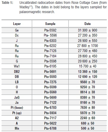
Radiocarbon dates (Table 1) imply several hiatuses, preceded and followed by pulses of intense occupation. The hiatus between ~2.2 kya and 6.0 kya demonstrates a sedimentary unconformity spanning a great portion of the middle and late Holocene. Another substantial hiatus occurs between layers G and DB2, although in parts of the cave a gritty orange wash dated ~15.7 kya separates the two layers.
Because of the dates and the relative densities of archaeological material, Wadley17(p.440) suggested that some of the darker organic-rich layers (e.g. Pt, H and DB) were slowly deposited during periods of gentle rainfall as shallow lenses with considerable anthropogenic content, while the underlying orange sands (e.g. CM to Ja and Wa1) accumulated rapidly and with less anthropogenic material. The latter were primarily formed through weathering or rock spalling of the sandstone roof and through material washed into the cave by springs, occasionally activated during protracted, heavy rains.25
To accurately contextualise all the palaeomagnetic results that will be discussed below, two charcoal samples were collected and submitted for accelerator mass spectrometry radiocarbon assays. The samples were processed by the Poznań Radiocarbon Laboratory, Poland. The new results obtained are given in Table 2. The date Poz-64224 (9500±50 BP) from layer Ja (the contents of which are attributed to the Oakhurst Industry), is somewhat older than the two dates (8380±70 and 8160±70 BP) previously obtained for layer Ja. The new date suggests that the entire Oakhurst sequence may be of greater antiquity than was previously thought.

Palaeomagnetic research
Sampling procedures
The palaeomagnetic samples (n=92) were taken from the fine sediments of the southern profile exposed by Wadley's excavations (Figure 2d). The profile reveals fine sediments with interbedded thin lenses of ashes, coarse-grained elements, and rock fall from the cave's roof. The orange sand, and intercalated lenses and levels of grey and/or rubefied material, testify to the presence of significant combustion phenomena, such as fireplaces. The samples - labelled RC together with a number - were vertically taken after carefully cleaning the section, then trying to follow the apparently undisturbed layers suitable for our research. Despite this it was difficult to attribute each sample precisely to the previously described stratigraphy. Samples were taken from layers A to DB as follows: samples RC1 to RC26 were generically from A and A2 corresponding to the Late Holocene, and RC28 to RC80 from levels Pt, Ja, H, CM and DCM. According to radiocarbon assays, they mainly belong to the Middle, Early Holocene (8-9.5 kya), and probably the Pleistocene-Holocene transition (~10.0/11.0 kya). Finally, the samples RC81 to RC92 came from the terminal Pleistocene DB and DB2 greenish sands which were dated at ~13-12 kya. We did not collect sediment between samples RC48 and RC49 at 74.0 cm and 79.0 cm depth, because sediments here were highly compacted by rubefaction. The date of 1.1 kya was obtained next to RC13 and RC14, corresponding to layer A, and the 9.5 kya assay was obtained close to RC44 and RC45, in the transition between the orange sand (layer Ja) and a compacted orange-grey sand with hearths embedded (layer Ph).
The cores were taken using 25-mm long and 20-mm diameter cylindrical PVC plastic containers. The cylinders were carefully pushed into the sediments, overlapping each other by about 50%. The sample's orientation was measured using a Brunton compass. Samples were consolidated with sodium silicate once removed and they were numbered from the top to the bottom. The depth of each sample is recorded in Supplementary table 1. Seven samples were taken for rock magnetic analysis nearby the location of palaeomagnetic samples.
Rock magnetic study
In previous work carried out by Herries and Latham11,12 on magnetic properties in Rose Cottage Cave, they found that the frequency dependence of magnetic susceptibility between unburned and burned sediments was very small. They determined this using a susceptibilimeter (Bartington) of two frequencies (460 Hz and 4600 Hz). In our studies we used a Kappabridge AGICO of three frequencies (1000 Hz, 4000 Hz and 16 000 Hz) and we also measured the dependence of the susceptibility at high (room temperature to near 700 °C) and low (room temperature to near -190 °C) temperatures. This allowed us to better discriminate the burnt sediments from the unburned ones.
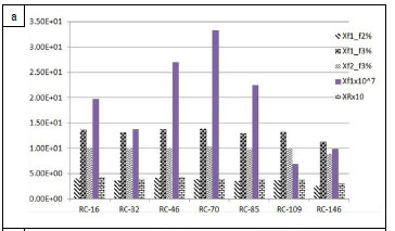
In order to characterise the magnetic mineralogy, we took seven samples catalogued as RC at respective depths of -16, -32, -46, -70, -85, -109 and -146 cm below surface. They were analysed with an AGICO MFK1-FA by using the variation of susceptibility (k) with temperatures from -190 °C to 700 °C, and the variation of susceptibility with applied fields from 10 A/m to 700 A/m at 1000 Hz; 10 A/m to 350 A/m at 4000 Hz and 10 A/m to 200 A/m at 16 000 Hz.
The variation of initial magnetic susceptibility with frequency was used as an indicator of superparamagnetic (SP) magnetite grains.26,27 It is indicated as X fL_fH% = 100 x [(XfL - XfH)/ XfL], where fL is the low frequency and fH the higher frequency. Frequencies are f1 = 1000 Hz, f2 = 4000 Hz and f3 = 16 000 Hz. Another parameter we used was proposed by Hrouda27 as XR = (Xf1 - Xf2)/ (Xf2 - Xf3 ). According to Hrouda: 'The advantage of the XR parameter is that it is not affected by any mineral fraction being frequency independent.' It can be used to estimate the size of the superparamagnetic grains, keeping in mind that its distribution follows a lognormal distribution.28,29 According to this and the data shown in Figure 3a, Hrouda's27 calculations show an estimate of grain size diameter for superparamagnetic particles in the range between between 39 nm and 11 nm (1 nm= 10-9 m). It is in agreement with the presence of very stable single mains, higher than 30 nm at room temperature, which are good magnetic remanence carriers.
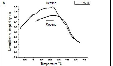
Typical magnetic susceptibility versus temperature curves are depicted in Figure 3b. It can be seen that there is a steady linear increase of susceptibility from near -180 °C to 125 °C that could be related to unblocking of superparamagnetic to single domain grains of Ti-poor magnetite and/or maghemite. There is no evidence of Verwey transition near -155 °C, so multidomain pure magnetite is absent in these samples. Heating curves show a Ti-poor magnetite Curie temperature near 575 °C, and a Curie temperature appropriate for haematite that perhaps formed as a byproduct when the hearths heated nearby strata. Due to the low magnetisation saturation of the haematite when compared with the Ti-poor magnetite or maghemite, it does not contribute significantly to the final remanence in these samples. Figure 3c depicts the low temperature susceptibility measurements of all the samples. The slope is related to the stable single domain/superparamagnetic transition because the blocking volume is proportional to temperature,28,29 so when the temperature increases, more magnetic grains go from stable single domain to superparamagnetic and the susceptibility increases. Sample RC-70 shows the higher slope, indicating a higher concentration of very fine superparamagnetic fraction; this finding can be related to sediments that suffered burning or higher combustion temperatures, or use of the site for a longer time. Samples RC-16 to RC-85 exhibits a similar slope, while in RC-109 and RC-146 the slope is very low, suggesting that these samples were not affected by a combustion event. This is in agreement with the results of the frequency dependence section, where a very fine superparamagnetic particle is predicted due to a broad grain size distribution.
In conclusion, the strata with burnt sediments as observed in samples RC-16 to RC-85 show stable single domain and superparamagnetic particles of Ti-poor magnetite, together with haematite, which is compatible with chemical processes during heating in situ of iron-bearing minerals. The magnetisation of saturation in haematite is 100 times lower than in Ti-poor magnetite. Therefore, the remanence recorded here is carried mainly by Ti-poor magnetite grains. Only when the concentration of Ti-poor magnetite is very low, can haematite be considered as a magnetic carrier. In this case, magnetic measurements show that Ti-poor magnetite is the main magnetic remanent carrier. Stable single domain grains are very stable magnetic carriers, so these sediments are suitable for recording ancient magnetic fields acquired during burning. Samples RC-109 and RC-146 do not exhibit high superparamagnetic content, suggesting that no burning events affected these sediments.
Remanence directions analysis and results
All samples were subjected to detailed stepwise alternating field demagnetisation in progressive steps of 3, 6, 9, 12, 15, 20, 25, 30, 40 and 60 mT with a three-axis static degausser attached to a 2G cryogenic magnetometer (755R). Additional steps of 80 mT and 100 mT were used for some specimens. The RC samples showed a common pattern with highly reliable magnetic behaviour. Most specimens had a gradual decrease of magnetisation with almost all remanence erased at 25 mT (RC2; Figure 4b), but mostly at 50 mT and 60 mT (RC1, 5, 8, 11, 15, 18, 24, 37, 54, 59, 61, 66, 75, 91; Figure 4a, c-l, n-o, q-s, v); 10% remains at 30 mT (e.g. R44; Figure 4k), 40 mT (e.g. RC60; Figure 4p), while a few indicate a drop at 80-100 mT (RC40, 47, 51, 83, 90; Figure 4j, l, m, t-u). As seen in the previous section, these differences are related to the magnetic carriers of the remanence.
Palaeomagnetic directions were determined by the 'Remasoft 3.0 palaeomagnetic data browser and analyser' computer program. The characteristic remanent magnetisation directions were calculated using principal components analysis. In most cases, the characteristic remanent magnetisation trended towards the coordinate's origin in the Zijderweld30 diagrams (Figure 4). The RC samples display varied patterns of behaviour in the vector diagram's projection. Some exhibit univectorial projections (RC1, 5, 24, 91; Figure 4a, c, h, v), while many have two magnetic components with one decaying to the origin (RC2, 11, 18, 40, 47, 51, 59, 61; Figure 4b, e, g, j, l-m, o, q). A viscous secondary component was easily removed in a number of specimens (RC2, 15, 40, 47, 51, 59, 66, 90; Figure 4b, f, j, l, m, o, r, u) between 3 mT and 12 mT and was not considered further. In a few specimens (e.g. RC40; Figure 4j), some scatter is observed when fitting the steps of demagnetisation to the origin of coordinates, probably due to the minor haematite presence (as recognised by rock magnetic experiments). Also, samples RC15, RC44 and RC90 do not go to the coordinates' origin of the orthogonal diagrams, but in these cases their harder component is similar to that obtained by samples decaying to the origin (Figure 4f, k,u). There were also several cores that recorded two geomagnetic field directions. As described in Supplementary table 2, the secondary ('soft') component in five samples recorded a normal position (e.g. RC11, 18; Figure 4e,g), but also an 'anomalous' direction in two specimens (e.g. RC75; Figure 4s); the 'hard' magnetisation is interpreted as an early remanence acquired during formation of the sedimentary deposit (e.g. RC11; Figure 4e). Finally, several cores recorded three magnetic components, one of which appears to decay to the origin (e.g. RC83; Figure 4t).
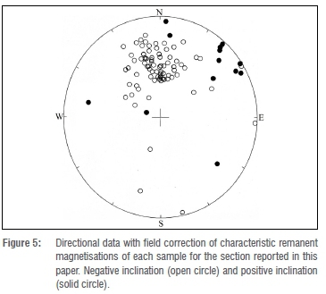
Many samples presented either a high (e.g. RC66; Figure 4r) or a low (e.g. RC60; Figure 4p) negative, and positive (e.g. RC11, RC40; Figure 4e, j) inclinations. Most specimens yielded a normal position (RC8, 15, 18, 90, 91; Figure 4d-e, u-v); a few samples showed northwesterly (RC2, RC15; Figure 4b, f), northeasterly or easterly (RC47, 60, 83; Figure 4l, p, t) directions, several of which had steep inclinations (RC60; Figure 4p). 'Anomalous' southward directions were found in various cores, mainly in the lower portion (RC40; Figure 4j). The number and intervals of the demagnetisation steps used to isolate the characteristic remanent magnetisation are given in Supplementary table 1, which also depicts the maximum angular deviations that generally have low values, ranging from 0° to 5° (n=82, 89.13%), and from 5.1° to 10° (n=10, 10.87%). This analysis shows that the RC samples mostly display normal, but also intermediate and reverse magnetic remanence of low negative and positive inclination values. Figure 5 illustrates the stereographic projection of characteristic remanent magnetisation for the RC sampling.
The magnetograms of the declination and inclination profile (Figure 6) exhibit wide amplitude fluctuations both in declination and inclination in the upper and lower portions of the section. In the former, directions vary widely with transitional positions gradually changing to normal from samples 1 to 19. Despite directional variations, with the exception of RC11, the inclination values are quite constant and normal directions with little difference from the present geomagnetic field occur up to RC39. It is noteworthy that there is a stable record with normal directions between samples RC19 to RC39, and a highly fluctuating log from RC39 to RC61 which is depicted with pointed lines and marked with arrows. Samples RC38 to RC41 show similar directions, but with a pronounced swing of ~130° to a positive inclination in RC40. Between RC45 and RC54, the samples exhibit similar inclination, but with varying directions, and with a deviation of ~180° from the normal geomagnetic field. Between samples RC53 and RC58, there is a strong swing both in declination and inclination values with transitional normal-reverse-normal positions, which in the latter are observed in samples between RC85 and RC92. As seen in Figure 6, the resulting logs show an important difference of ~50-60° in inclination in the period ~≥9.5 kya.

After checking that the directional data from Rose Cottage were useful for assessing a Fisherian distribution, the site mean directions were computed (Figure 7).

Additionally, the mean direction was calculated by segmenting the Rose Cottage record according to the most frequent directional changes observed in its upper, middle and lower portions (Supplementary table 3). From this study, it is observed that Rose Cottage mean directions show a consistent agreement; they are also located close to the International Geomagnetic Reference Field direction (D=337.4°, I=-63.9°) for 2014, the year in which the sampling was performed. However, a significant difference is observed for the mean directions calculated in the upper and lower portion of the section (Figure 7).
The virtual geomagnetic pole positions were calculated from the aforementioned directions (Supplementary table 1, Figure 8a). When plotted on a present world map, besides normal positions, virtual geomagnetic pole positions show intermediate and reverse positions from the rotation axis of the earth (Figure 8b). The virtual poles in the northern hemisphere are located in North America, Greenland, and north, east and southeastern Asia, and northern South America. Virtual geomagnetic pole positions in the southern hemisphere are situated in Indonesia, South of the Pacific Ocean, and west of southern Africa; those ones calculated from secondary directions are located close to New Zealand. Surprisingly, virtual geomagnetic pole position locations from Rose Cottage show a remarkable agreement with those calculated from Klasies River Cave 1.14(Fig.8) Interestingly, as seen in Figure 8b-f, virtual geomagnetic pole positions from Rose Cottage show consistency between the locations observed in other places during the Pleistocene-Holocene transition and Holocene.31,32Virtual geomagnetic pole positions located in the above-mentioned positions, mainly near the Americas and Australasia, attract attention because they agree with the transitional longitudinal bands registered in excursions and polarity transitions in different parts of the world since the early Jurassic.33 Also they coincide with present-day zones of fast seismic velocity at the core-mantle boundary.34

Discussion and conclusion
Palaeomagnetic data obtained in the fine-grained sediments from a section at Rose Cottage have mostly shown normal directions, especially between samples RC18 to RC39 and RC85 to RC92; however, some samples, principally from RC40 to RC84, exhibit 'anomalous' southward directions where wide pulses occurred at different times during the Early and Late Holocene. A significant westward shift in declination of ~80° can be observed, and a conspicuous fluctuating inclination in the lower part of the section during the Early Holocene at ≥9.5 kya, and after ~12.0/13.0 kya (Figure 6). The normal directions correspond to the palaeosecular variations record for South Africa during the time span under consideration. Most oblique directions far from the present geomagnetic field are located mainly in the lower portion of the upper sediments. Such palaeomagnetic records may be due to several reasons. Various issues can give rise to anomalous directions of remanent magnetism that do not reflect the true geomagnetic field behaviour, such as diverse deposition processes, chemical alterations as well as sedimentary physical disturbances35,36 and human error. If the directional data observed at Rose Cottage are not from any of the aforementioned causes, they correspond to the geomagnetic field record for southern Africa during the last millennia of the Pleistocene and Holocene.
As noted above, the Rose Cottage sedimentary stratigraphy is the result of episodic sedimentation37 registering a discontinuous record with gaps of ≥3.8 ky between ~2.2 kya and 6.0 kya, that is, during the Late and Middle Holocene. Despite discontinuities, the unstable directional logs suggest some instability during certain periods of the Holocene. The Rose Cottage oblique normal and oblique reverse samples exhibit several palaeomagnetic consistencies such as their location in the northeast quadrant of the stereoplot, something that also occurred at Klasies River Cave(Fig.5), South Africa. Fluctuating logs were also reported at a similar latitude to Rose Cottage in southern Brazil38, and northeastern Argentina, some of them with positive inclination values32,39. In other places in the southern hemisphere, low values, some with positive inclination, were recorded during very recent times in the Late Holocene.31(Fig.9-10),32,40,41 However, due to the larger number of specimens, our main focus is on the anomalous directions observed in the lower segment of the magnetograms with a direct date of ~9.5 kya corresponding to the Early Holocene. Hence, at this time the Rose Cottage record suggests that swings with wide amplitude variations in declination alternated between normal, intermediate and reverse positions. This suggests that the geomagnetic field might have anomalous behaviour in South Africa during the Pleistocene-Holocene transition and early Holocene. It is significant to point out that the current paradigm in palaeomagnetic research is that during this time, the geomagnetic field behaviour was normal as it is now.42,43 However, since the 1970s, a number of similarly aged records with anomalous directions were reported in samples taken from diverse materials, and environments in different parts of the world.31,32,44-56 Interestingly, samples from the Starnö core in Sweden, dated by varved chronology to 10 127-10 153 BC or 12 077-12 103 years BP, yielded virtual geomagnetic pole positions located in northern South America.44(Fig.9),47(Fig.2) Of importance, as seen in Figure 8d, almost all of the samples from the El Tingo site in Ecuador gave virtual geomagnetic pole positions located in southern Africa.55 A list of well-dated records of the possible excursion that occurred during the terminal Pleistocene/Early Holocene is given by Nami and colleagues56(Table 2). The inclinations have the expected values during the time span under consideration. Large amplitude swings in declination were recorded in Scandinavia and northern Russia.57,58 A similar situation was also registered in southernmost Patagonia at Potrok Aike lagoon; there the palaeosecular variation record yielded logs of negative inclination values with large amplitude variations in declination during the early Holocene at ~7-9 kybp.59 These large reverse pulses spanning short periods might alternate with normal geomagnetic field directions that might mask or cover up their existence in the palaeomagnetic record.
In summary, the Rose Cottage deposit can be interpreted as a preliminary palaeosecular variation record for South Africa. It shows significant directional changes in declination and inclination with intermediate and reverse virtual geomagnetic pole positions during the terminal Pleistocene and Holocene. Therefore, these results should be simply interpreted as chronostratigraphic tools. Hence, if the presented palaeomagnetic features are true geomagnetic field behaviour, the remarkable palaeosecular variation record can serve to correlate regional stratigraphies, and calibrate relative and absolute chronologies.1,5-7 Additionally, if the anomalous directions do represent an excursion, it may be used also as a dating device1,3,5-7, becoming an excellent magnetostratigraphic marker for the period spanning the Rose Cottage palaeomagnetic record.
Acknowledgements
The project 'Geomagnetic field excursions for Late Pleistocene-Holocene deposits in South Africa and Lesotho: Geoarchaeological and chronological implications for the Later and Middle Stone Age' was co-funded by the DST/NRF Centre of Excellence (CoE) in Palaeosciences and the Palaeontological Scientific Trust (PAST) with two research grants to Paloma de la Peña. The support of the CoE in Palaeosciences and PAST towards this research is hereby acknowledged. Opinions expressed and conclusions arrived at, are those of the authors and are not necessarily to be attributed to the CoE in Palaeosciences or PAST. The Evolutionary Studies Institute (University of the Witwatersrand), CONICET and Universidad de Buenos Aires provided logistical and technical support.
Authors' contributions
H.G.N. was responsible for conceptualisation, project leadership, methodological design, data collection, sample analysis and the write-up. C.A.V. was responsible for sample analysis and writing concerning rock magnetism. L.W. was responsible for validation and writing on the research. P.d.l.P. was responsible for conceptualisation, project leadership, project management, methodological design, data collection, the writing, and acquiring the funding (PAST and DST/NRF CoE).
References
1.Tarling DH. Palaeomagnetism: Principles and applications in geology, geophysics, and archaeology. New York: Chapman and Hall; 1983. http://dx.doi.org/10.1007/978-94-009-5955-2 [ Links ]
2.Stenberg RS. The geophysical basis of archaeomagnetic dating. In: Eighmy JL, Sternberg RS, editors. Archaeomagnetic dating. Tucson, AZ: University of Arizona Press; 1990. p. 5-28. https://doi.org/10.1002/gea.3340060405 [ Links ]
3.Merrill RT, McFadden PL. The use of magnetic field excursions in stratigraphy. Quat Res. 2005;63:232-237. http://dx.doi.org/10.1016/j.yqres.2005.02.007 [ Links ]
4.Laj C, Channel JET. Geomagnetic excursions. In: Kono M, editor. Treatise on geophysics. Amsterdam: Elsevier; 2007. p. 373-416. http://dx.doi.org/10.1016/b978-044452748-6/00095-x [ Links ]
5.Barendrest RW. Using palaeomagnetic remanence and magnetic susceptibility data for the differentiation, relative correlation and absolute dating of quaternary sediments. In: Mahaney WC, editor. Quaternary dating methods. Amsterdam: Elsevier; 1984. p. 101-140. http://dx.doi.org/10.1016/S0920-5446(08)70067-0 [ Links ]
6.Parkes PA. Current scientific techniques in archaeology. New York: St. Martin's Press; 1986. [ Links ]
7.Herz N, Garrison EG. Geological methods for archaeology. New York: Oxford University Press; 1998. [ Links ]
8.Van Zijl JSV, Graham KWT, Hales AL. The palaeomagnetism of the Stormberg lavas of South Africa. Geophys J R Astr Soc. 1962;7:23-29. [ Links ]
9.Hattingh PJ. Palaeomagnetism of the upper zone of the Bushveld Complex, Tectonophysics. 1989;165:131-142. https://doi.org/10.1016/0040-1951(89)90042-5 [ Links ]
10.Thackeray JF, Kirschvink JL, Raub TD. Palaeomagnetic analyses of calcified deposits from the Plio-Pleistocene hominid site of Kromdraai, South Africa. S Afr J Sci. 2002;98:537-540. [ Links ]
11.Herries AIR, Latham A. Environmental archeomagnetism: Evidence for climatic change during the later Stone Age using the magnetic susceptibility of cave sediments from Rose Cottage Cave, South Africa. In: Mitchell P, Haour A, Hobart J, editors. Researching Africa's past: New contributions from British archaeologists. Oxford: Oxford University School of Archaeology, Oxford University Press; 2003. p. 25-34. https://doi.org/10.1017/s0021853704219934 [ Links ]
12.Herries AIR. New approaches for integrating palaeomagnetic and mineral magnetic methods to answer archaeological and geological questions on Stone Age sites. In: Fairbairn A, O'Connor S, Marwick B, editors, New directions in archaeological science. Canberra: ANUE Press; 2009. p. 235-254. https://doi.org/10.22459/ta28.02.2009.16 [ Links ]
13.Herries AIR. Shaw J Palaeomagnetic analysis of the Sterkfontein palaeocave deposits: Implications for the age of the hominin fossils and stone tool industries. J Hum Evol. 2011;60:523-539. http://dx.doi.org/10.1016/j.jhevol.2010.09.001 [ Links ]
14.Nami HG, De la Peña P, Vásquez CA, Feathers J, Wurz S. Palaeomagnetic results and new dates of sedimentary deposits from Klasies River Cave 1, South Africa. S Afr J Sci. 2016;112(11/12), Art. #2016-0051, 12 pages. http://dx.doi.org/10.17159/sajs.2016/20160051 [ Links ]
15.Harper PT. The Middle Stone Age sequence at Rose Cottage Cave: A search for continuity and discontinuity [MA thesis]. Johannesburg: University of the Witwatersrand; 1994. [ Links ]
16.Harper PT. The Middle Stone Age sequence at Rose Cottage Cave: A search for continuity and discontinuity. S Afr J Sci. 1997;93:470-475. [ Links ]
17.Wadley L. Rose Cottage Cave: Archaeological work 1987 to 1997. S Afr J Sci. 1997;93(10):439-444. [ Links ]
18.Vogel JC, Marais M. Pretoria radiocarbon dates. Radiocarbon. 1971;1:387-394. https://doi.org/10.1017/s003382220000850x [ Links ]
19.Valladas H, Wadley L, Mercier N, Tribolo C, Reyss JL, Joron JL. Thermoluminescence dating on burnt lithics from Middle Stone Age layers at Rose Cottage Cave. S Afr J Sci. 2005;101:169-174. [ Links ]
20.Woodborne S, Vogel JC. Luminescence dating at Rose Cottage Cave: A progress report. S Afr J Sci. 1997;93:476-478. [ Links ]
21.Pienaar M, Woodborne S, Wadley L. Optically stimulated luminescence dating at Rose Cottage Cave. S Afr J Sci. 2008;104:65-70. [ Links ]
22.Wadley L. The Robberg Industry of Rose Cottage Cave, eastern Free State: The technology, spatial patterns and environment. S Afr Archaeol Bull. 1996;51:64-74. https://doi.org/10.2307/3888841 [ Links ]
23.Wadley L. The early Holocene layers of Rose Cottage Cave, eastern Free State: Technology, spatial patterns and environment. S Afr Archaeol Bull. 2000;55:18-31. https://doi.org/10.2307/3888889 [ Links ]
24.Wadley L. The Wilton and pre-ceramic post-classic Wilton industries at Rose Cottage Cave and their context in the South African sequence. S Afr Archaeol Bull. 2000;55:90-106. https://doi.org/10.2307/3888959 [ Links ]
25.Butzer KW. Archaeogeology and Quaternary environment in the interior of southern Africa. In: Klein RG, editor. Southern African prehistory and paleoenvironments. Rotterdam: Balkema; 1984. p. 1-64. [ Links ]
26.Worm HU. On the superparamagnetic-stable single domain transition for magnetite, and frequency dependence of susceptibility. Geophys J Int. 1998;133:201-206. https://doi.org/10.1046/j.1365-246X.1998.1331468.x [ Links ]
27.Hrouda F. Models of frequency-dependent susceptibility of rocks and soils revisited and broadened. Geophys J Int. 2011;187:1259-1269. http://dx.doi.org/10.1111/j.1365-246X_2011.05227.x [ Links ]
28.Vásquez CA, Orgeira MJ, Sinito AM. Origin of superparamagnetic particles in Argiudolls developed on loess, Buenos Aires (Argentina). Environ Geol. 2009;56(8):1653-1661. https://doi.org/10.1007/s00254-008-1262-8 [ Links ]
29.Vásquez CA, Sapienza FF, Somacal A, Fazzito SY. Anhysteretic remanent magnetization: Model of grain size distribution of spherical magnetite grains. Stud Geophys Geod. 2018;62(2):339-351. https://doi.org/10.1007/s11200-017-1233-1 [ Links ]
30.Zijderveld JDA. A. C. demagnetization of rocks: Analysis of results. In: Collinson DW, Creer KM, Runcorn SK, editors. Amsterdam: Elsevier; 1967. p. 254-286. [ Links ]
31.Nami HG. Possible Holocene excursion of the earth's magnetic field in southern South America: New records from archaeological sites in Argentina. Earth Planet Space. 1999;51:175-191. http://dx.doi.org/10.1186/BF03352222 [ Links ]
32.Nami HG. New detailed Holocene paleomagnetic records with anomalous geomagnetic field behavior in Argentina. Geoacta. 2012;37(2):83-116. [ Links ]
33.Vizán H, Van Zele MA. Jurassic-Early Cretaceous intermediate virtual geomagnetic poles and Pangaean subduction zones. Earth Planet Sci Lett. 2008;266(1-2):1-13. http://dx.doi.org/10.1016/j.epsl.2007.09.044 [ Links ]
34.Vizán H, Mena M, Vilas JF. Pangea, the geoid and the paths of virtual geomagnetic poles during polarity reversals. J South Am Earth Sci. 1993;VI(4):253-266. https://doi.org/10.1016/0895-9811(92)90045-z [ Links ]
35.Verosub K, Banerjee SK. Geomagnetic excursions and their paleomagnetic record. Rev Geophys. 1977;15:145-155. http://dx.doi.org/10.1029/RG015i002p00145 [ Links ]
36.Langereis CG, Van Hoof AAM, Rochette P. Longitudinal confinement of geomagnetic reversal paths as a possible sedimentary artifact. Nature. 1992,358:228-230. http://dx.doi.org/10.1038/358226a0 [ Links ]
37.Dott RHJ. Episodic sedimentation - How normal is average? How rare is rare? Does it matter? J Sediment Petrol. 1983;53:5-23. https://doi.org/10.1306/212f8148-2b24-11d7-8648000102c1865d [ Links ]
38.Santos NO, Savian JF, Hartmann GA, Trindade RIF, Toldo EE, Ivanoff MD, et al. Análise preliminar de variações de campo magnético em registros sedimentares da Lagoa dos Patos, Rio Grande do Sul, Brasil [Preliminary analysis of magnetic field variations in sedimentary records of Lagoa dos Patos, Rio Grande do Sul, Brazil]. Latinmag Lett. 2016;6(Special Issue C13):1-5. Proceedings São Paulo, Brazil. Portuguese. Available from: http://www.geofisica.unam.mx/LatinmagLetters/LL16-01-SP/C/C13.pdf
39.Sinito AM, Gogorza C, Nami HG, Irurzun MA. Observaciones Paleomagnéticas en el Sitio Arqueológico Puerto Segundo (Misiones, Argentina) [Paleomagnetic Observations in the Puerto Segundo Archaeological Site (Misiones, Argentina)]. An Asoc Fís Arg. 2001;13:237-241. Spanish.
40.Nami HG. Preliminary paleomagnetic results of a terminal Pleistocene/Holocene record from northeastern Buenos Aires province (Argentina). Geofizika. 2006;23(2):119-141. [ Links ]
41.Nami HG. New detailed paleosecular variation record at Santa Lucía archaeological site (Corrientes province, northeastern Argentina). Geofís Int. 2011;50(2):9-21. [ Links ]
42.Donadini F. Features of the geomagnetic field during the Holocene and Proterozoic. Report Series in Geophysics 52. Helsinki: University of Helsinki; 2007. [ Links ]
43.Barletta F, St-Onge G, Channell JET, Rochon A. Dating of Holocene western Canadian Arctic sediments by matching paleomagnetic secular variation to a geomagnetic field model. Quat Sci Rev. 2010;29:2315-2324. https://doi.org/10.1016/j.quascirev.2010.05.035 [ Links ]
44.Nöel M. The paleomagnetism of varved clays from Blekinge, southern Sweden. Geol Tor Stockholm Forhandl. 1975;97:357-367. https://doi.org/10.1080/11035897509454326 [ Links ]
45.Olausson E, Svenonius B. Force and polarity of the terrestrial magnetic field during the last 20,000 years. Geol För Stockholm Förh. 1974;96:321-325. https://doi.org/10.1080/11035897409454286 [ Links ]
46.Thompson R, Kelts K. Holocene sediments and magnetic stratigraphy from Lakes Zug and Zurich, Switzerland. Sedimentology. 1974;21(4):577-596. https://doi.org/10.1111/j.1365-3091.1974.tb01791.x [ Links ]
47.Noël M, Tarling D. The Laschamp geomagnetic event. Nature. 1975;253:705-707. https://doi.org/10.1038/253705a0 [ Links ]
48.Creer KM, Anderson TW, Lewis CFM. Late Quaternary geomagnetic stratigraphy recorded in the Lake Erieu sediments. Earth Planet Sci Lett. 1976;31:37-49. https://doi.org/10.1016/0012-821x(76)90094-7 [ Links ]
49.Mörner NA. The Gothenburg magnetic excursion. Quat Res. 1977;7(3):413-427. https://doi.org/10.1016/0033-5894(77)90031-x [ Links ]
50.Geiss CE, Banerjee SK. A Holocene-Late Pleistocene geomagnetic inclination record from Grandfather Lake, SW Alaska. Geophys J Int. 2003;153:497-507. https://doi.org/10.1046/j.1365-246x.2003.01921.x [ Links ]
51.Lund SP, Platzman E, Thouveny N, Camoin G. Evidence for two new paleomagnetic field excursions ~2,500 and ~12,500 years ago from the South Pacific Ocean Region (Tahiti). Eos Trans AGU. 88(52 Suppl.):GP42A-05. Available from: http://abstractsearch.agu.org/meetings/2007/FM/GP42A-05.html [ Links ]
52.Lund SP, Platzman E, Thouveny N, Camoin G, Yokoyama Y, Matsuzaki H, et al. Evidence for two new magnetic field excursions (11,000 and 13,000 Cal Yrs BP) from sediments of the Tahiti Coral Reef (Maraa tract). Eos Trans AGU. 2008;89(53 Suppl.):GP21B-0786. Available from: http://abstractsearch.agu.org/meetings/2008/FM/GP21B-0786.html [ Links ]
53.Nelson FE, Wilson GS. Shipboard party. Environmental magnetism and excursion record of the Pleistocene-Holocene transition in marine cores, West Coast South Island, New Zealand. Geophys Res Abstracts. 2009;11, EGU2009-430. [ Links ]
54.Chaparro MAE, Böhnel HN, Byrne R, Nowaczyk NR, Molina-Garza RS, Parkand Jörg J, et al. Palaeomagnetic secular variation and rock-magnetic studies of Holocene sediments from a maar lake (Hoya de San Nicolas) in Central Mexico. Geophys J Int. 2008;175(2):462-476. https://doi.org/10.1111/j.1365-246x.2008.03893.x [ Links ]
55.Nami HG. Detailed paleomagnetic records from Ecuador and new evidence for the geomagnetic field excursion during the Late Pleistocene-Holocene. Geofis Int. 2015;54:127-148. https://doi.org/10.1016/j.gi.2015.04.009 [ Links ]
56.Nami HG, Vásquez CA, Durán VA. Detailed early Holocene (10.3 cal kybp) paleomagnetic record with anomalous directions from Mendoza Province, Western Argentina. Latinmag Lett. 2017;7:1-17 LL17-0702Rs. [ Links ]
57.Bakhmutov V. Secular variations of the geomagnetic field, indicated in Early Holocene deposits of Lake Ladoga. Geophys J. 1997;16:481-498. [ Links ]
58.Saarnisto M, Saarinen T. Deglaciation chronology of the Scandinavian Ice Sheet from the Lake Onega Basin to the Salpausselkä End Moraines. Global Planet Change. 2001;31:387-405. https://doi.org/10.1016/s0921-8181(01)00131-x [ Links ]
59.Gogorza C, Irurzun A, Sinito AM, Lisé-Pronovost A, St-Onge G, Haberzettl T, et al. High-resolution paleomagnetic records from Laguna Potrok Aike (Patagonia, Argentina) for the last 16,000 years. Geochem Geophys. 2012;13:1. https://doi.org/10.1029/2011gc003900 [ Links ]
60.Nami HG. Holocene geomagnetic excursion at Mylodon Cave, Ultima Esperanza, Chile. J Geomag Geoelect. 1995;47:1325-1332. http://dx.doi.org/10.5636/jgg.47.1325 [ Links ]
 Correspondence:
Paloma de la Peña
paloma.delapenya@gmail.com
Received: 08 July 2019
Revised: 04 Sep. 2019
Accepted: 09 Sep. 2019
Published: 29 Jan. 2020
Editor: Maryna Steyn
Funding: DST/NRF Centre of Excellence in Palaeosciences, Palaeontological Scientific Trust (PAST)
Supplementary Material
The supplementary file is available in pdf: [Supplementary file]

