RESEARCH ARTICLE

 

Spatial variability of PM₁₀, PM_2.5 and PM chemical components in an industrialised rural area within a mountainous terrain

 

 

Cheledi Tshehla^{I, II}; Caradee Y. Wright^{I, III}

^IDepartment of Geography, Geoinformatics and Meteorology, University of Pretoria, Pretoria, South Africa
^IISouth African Weather Service, Pretoria, South Africa
^IIIEnvironment and Health Research Unit, South African Medical Research Council, Pretoria, South Africa

Correspondence

 

 

---

ABSTRACT

We describe the measurement and spatial variability of particulate matter (PM) chemical composition, PM₁₀ and PM_2.5 in the Greater Tubatse Municipality, South Africa. Monthly samples were collected over 12 months (July 2015 to June 2016) using the inexpensive and easy to operate passive samplers of the University of North Carolina. Sites for sample collection were located at private residences, a church, a hospital and a school. Concentrations of PM₁₀, PM_2.5 and PM chemical components were determined using computer-controlled scanning electron microscopy with energy-dispersive X-ray spectroscopy. The annual observed concentrations at all sites were below the South African National Ambient Air Quality Standards of 40 µg/m³ for PM₁₀ and 25 µg/m³ for PM_2.5. The Cr-rich and CrFe-rich particles showed substantial heterogeneity with high concentrations observed near the chrome smelters, and Si-rich particles were highest near the silicon mine. SiAl-rich particles were highest at sites close to busy roads, while SiAlFe-rich particles were less spatially distributed. The low spatial variability of SiAlFe-rich particles indicates that these elements are mainly found in crustal material. Using the synoptic meteorological parameters of The Air Pollution Model, we were unable to effectively determine correlations between PM₁₀ and mixing height, Monin-Obukhov length, air pollution potential, or coefficient of divergence.
SIGNIFICANCE:
•We have shown that the use of University of North Carolina passive samplers coupled with computer-controlled scanning electron microscopy is effective in determining the chemical composition of PM.
•The use of passive samplers is a cheap and effective method to collect data in remote areas of South Africa which have limited or no electricity supply.
•Assessment of the spatial distribution of PM and PM chemical components can assist in the development of effective air quality management strategies

Keywords: complex terrain, passive samplers, mixing height, air pollution potential

---

 

 

Introduction

Airborne particulate matter (PM) is a term used to describe solid particles or a mixture of solid and liquid droplets suspended in the air.¹ The particle mixture may vary in size distribution, composition and morphology and may be in the form of sulfates, nitrates, ammonium and hydrogen ions, trace elements (including toxic and transition metals), organic material, elemental carbon (or soot) and crustal components.^2,3 PM may originate from either primary or secondary sources. Primary particles are those directly emitted into the atmosphere from sources such as road vehicles, coal burning, industry, windblown soil, dust and sea spray. Secondary particles are particles formed within the atmosphere by chemical reactions or condensation of gases. The major contributors of secondary particles are sulfate and nitrate salts formed from the oxidation of sulfur dioxide and nitrogen oxides, respectively.⁴ Ambient PM has long been associated with adverse effects on respiratory, cardiovascular and cardiopulmonary health.^5-7 The severity of such health effects depends largely on the size, concentration and composition of inhaled particles.⁸ PM pollution emanating from industrialisation has serious environmental impacts mainly because of the release of toxic substances and trace metals into the atmosphere.⁹

Industrialisation and urbanisation of rural areas can lead to the emission of large amounts of PM and chemical elements into the atmosphere. These emissions result in widespread air pollution problems¹⁰, and these problems have proved to be more regional and complex with time¹¹. The Greater Tubatse Municipality (GTM) in South Africa is home to a large number of people and a variety of anthropogenic pollution sources such as chrome smelters, mines (for chrome, silicon and platinum), agricultural operations, biomass combustion, brick manufacturing, vehicles and unpaved roads, which can contribute to PM emissions. Differences in the composition of particles emitted by these sources may lead to spatial heterogeneity in the composition of the atmospheric aerosols. Hence, understanding the spatial variability of PM is of great importance for environmental planning and management purposes by both the industries and governing authorities. Therefore, this study will lay a foundation for developing effective intervention strategies to reduce PM emissions in the GTM. In South Africa, PM is only regulated in two size fractions (PM₁₀ and PM_2.5). However, to date, there are no ambient air quality standards for elemental particles. The list of metals regulated under the National Environmental Management: Act No. 39 of 2004 should be expanded to include metals such as chromium, iron, arsenic, copper, cobalt, manganese and other metals that have been identified¹² to have the potential to cause environmental health threats.

Apart from air pollution challenges due to anthropogenic activities, South Africa has a varying topography ranging from flat to complex terrain that can have differing effects on the dispersion of air pollutants. The shape of the landscape plays an important role in trapping or dispersing pollutants. Air pollution in mountain valleys tends to be higher in colder months than in warmer months.¹³ The distribution of pollutants depends largely on the meteorology and the landscape of the area. Surface heterogeneity plays a major role in the interaction between the atmosphere and the underlying surface, and it affects moist convection, and systematically produces responses in both local circulation and regional climate.^14-18 Complex terrain such as that of the GTM is characterised by high mountains and steep inclinations. In this type of terrain, the wind flow is very hard to predict. However, the steep slopes give rise to thermally induced circulations like mountain valley breezes which strongly modify the characteristics of synoptic flow.^19-22 The ability of the atmosphere to disperse pollutants depends on the local circulations, mixing height, stability of the atmosphere and wind strength. However, the complex nature of the terrain in the GTM and the lack of electricity supply in some areas of the municipality, makes it impossible to rely only on a network of continuous ambient air pollution monitoring.

A number of methods have been developed over the years to collect and analyse air pollutant samples, using both active and passive techniques. The passive sampling techniques involve non-active means such as gravitational settling to collect air samples onto the substrate. This method of sampling is cheaper than active sampling and allows for the deployment of more samplers to evaluate air pollution spatially.²³ The GTM has only one air quality monitoring station that is not sufficiently well maintained to produce good quality data. As a result, a network of passive samplers was used to determine the spatial variation of PM_2.5 and PM₁₀, which in future can be used as a baseline for the deployment of active samplers in the area.

Mountain winds

Wind circulations in the free atmosphere above the mountains and valleys are governed by pressure gradients between large circulation systems.²⁴ The lower troposphere interacts with mountains, valleys and vegetation that in turn alter the circulation patterns. Mountainous terrain has a high degree of topographical variation and land-cover heterogeneity.²⁵ This variation in topography influences the atmosphere in two ways.²⁶ The first is in the form of momentum exchange between the atmosphere and the surface that occurs as a result of flow modification by mountains in the form of mountain lee waves, flow channelling and flow blocking.²⁷ The second effect involves energy exchange between the terrain and the atmosphere. The thermally induced winds depend on the temperature differences along the mountain plains systems and the strength of the synoptic systems and the cloud cover, with weak synoptic systems and cloud-free atmosphere producing more pronounced winds.^20,28 Mountain winds blow parallel to the longitudinal axis of the valley, directed up-valley during daytime and down-valley during night time. The circulation is closed above the mountain ridges by a return current flowing in the reverse direction. The actual development of thermally driven winds is often complicated by the presence of other wind systems developed on different scales.^22,28 Anabatic flows are more temporally limited during wintertime than summertime due to the shorter exposure period to sunlight.²⁹

Mixing height

Mixing height (MH) is the height to which relatively vigorous mixing occurs in the lower troposphere. Temperature inversions are most common in mountainous terrain where cool mountain air sweeps down into the valley at night, below the warm, polluted air. This inversion keeps the emitted pollutants close to the ground instead of allowing them to disperse into the atmosphere. A flow of thermal or synoptic origin channelled inside a mountain valley can transport plumes along the valley floor, thus limiting crosswind dispersion. Pollution stagnation in the bottom of the valleys can be favoured by the temperature inversion that develops inside the valley during the night and is destroyed by the growing convective boundary layer in the morning.³⁰ The thermally induced MH influences the concentration and transport of pollutants³¹, and is used in air quality models to determine atmospheric pollutant dispersion^32-34. However, in mountainous terrain, processes such as MH and mountain slope winds are coupled together³⁵ to transport air pollutants across mesoscales to synoptic scales³⁶. Research by De Wekker and Kossmann²⁷ has illustrated that the dispersion of pollutants in mountainous terrain does not depend on the boundary layer but rather on the thermally induced mountain slope winds.

Monin-Obukhov length

The Monin-Obukhov (MO) similarity theory has been applied in air pollution modelling for determining the dispersion of air pollutants. The MO measures the stability of the atmosphere, with stable atmospheric conditions favouring higher pollutant concentrations and unstable conditions allowing the dispersion of pollutants and hence lowering pollutant concentrations.³⁷ However, the MO is restricted to horizontal homogeneous terrains where there are no sudden roughness changes (such as in forested area, hilly or mountainous terrain) to modify the velocity profile and turbulent transport of heat and momentum.³⁸ Figueroa-Esspinoza and Salles³⁸ and Grisogono et al.³⁹ reported that MO theory is unable to account for the transport of pollutants in mountain valleys because the flow dynamics of the valleys are governed by anabatic and katabatic flows. These flows are generated by the mountain slopes and are normally decoupled from the synoptic flows above.

Ventilation coefficient

Gross⁴⁰ defined the ventilation coefficient (VC) as the product of the MH and the average wind speed, which can also be defined as a measure of the volume rate of horizontal transport of air within the MH per unit distance normal to the wind. Iyer and Raj⁴¹ describe the VC as a measure of the atmospheric condition that gives an indication of the air quality and air pollution potential. When the coefficient is higher, it is an indication that the atmosphere is able to disperse air pollutants effectively, resulting in a better state of air quality, whereas low ventilation indicates poor pollutant dispersion resulting in high pollution levels. The VC varies diurnally during summer and winter with high coefficients observed in the late afternoon and low values in the early mornings. Winter coefficients are also lower than those in summer due to low MH and reduced wind speeds in winter,^42,43 and the influence of the dominant anti-cyclones that are experienced over southern Africa during the winter months.

Air pollution potential

Gross⁴⁰ and Nath and Patil⁴⁴ describe air pollution potential (APP) as the measure of the inability of the atmosphere to adequately dilute and disperse pollutants emitted into it. The APP depends on meteorological conditions such as the MH, wind speed, atmospheric stability and solar radiation.⁴⁵ Once the pollutants are emitted into the atmosphere, their transportation is dependent on the mean wind speed which carries the pollutants away from the source to their sinks, and their convective mixing is dependent on the vertical temperature gradient.⁴⁴ The higher values of APP indicate that the atmosphere is unfavourable for the dilution and dispersion of pollutants⁴⁶ and indicate high concentrations of observed pollutants at the receiving environment. The low values of APP indicate that the atmosphere is conducive for the dispersion of pollutants which will result in low concentrations on the receiving environment.⁴⁴ The APP can be used as a management tool for siting of ambient air quality monitoring stations and for land-use planning in the development of new residential areas and zoning of new industrial sites.

The aim of this work was to determine the spatial variability of PM₁₀, PM_2.5 and PM chemical composition. Further analysis of the MO theory, MH, VC and the atmospheric pollution potential was performed to determine whether these factors have any influence on the PM₁₀ concentrations in the study area.

 

Methods

Study area

Sampling of PM was undertaken in a rural area of the GTM in Limpopo Province, South Africa (Figure 1). The main towns in the area are Steelpoort and Burgersfort which are sustained through economic activities such as mining and smelting of chromium ores. Furthermore, there are agricultural and forestry activities and transportation that also add to the economic activities in the area. Most of the households in the area are dependent on wood burning for space heating and cooking. The GTM has a complex terrain with high mountains and steep inclinations. The elevation of the surface area is approximately 740 m above sea level with the surrounding mountains extending to a height of approximately 1200-1900 m above sea level. The area is located in the subtropical climate zone where the maximum and minimum average temperatures are 35 °C and 18 °C, respectively in summer, and 22 °C and 4 °C, respectively in winter.⁴⁶ The annual rainfall for the area ranges between 500 mm and 600 mm.⁴⁷

Site selection

The locations of the monitoring sites were selected to optimise spatial sampling for exposure assessment. A sequential sampling technique^48,49 was used to design an optimal sampling network of six sites in the GTM. This technique is based on extended knowledge of the area to be sampled and factors controlling the distribution of pollutants. These factors could be the terrain and various phenomena like meteorological conditions and the chemistry of pollutants.⁵⁰ The number of sites selected was influenced by budgetary constraints due to costs associated with laboratory analysis of samples. The sites were located at private residences, a church, a hospital and a school, to ensure a secure area with easy access for site visits.

Sampling and sample analysis

The University of North Carolina passive samplers designed by Wagner and Leith²³ and housed in a protective shelter designed by Ott et al.⁵¹ were deployed at six sites for PM sampling. Ott et al.⁵¹ designed the shelter to shield the passive sampler from precipitation and to minimise the influence of wind speed on particle deposition.⁵² The samplers consist of a scanning electron microscopy stub, a collection substrate and a protective mesh cap.⁵³ The samplers were deployed for a period of ±30 days from July 2015 to June 2016, except for the months of August-September and September-November for which they were deployed for a period of >35 days. The longer sampling periods were selected to ensure that there was sufficient particle loading on the samplers.⁵²

The PM_2.5 and PM₁₀ concentrations and the elemental composition of individual particles deposited on the passive sampler were determined by computer-controlled scanning electron microscopy with energy-dispersive X-ray spectroscopy (CCSEM-EDS). Before sample analysis by photoemission electron microscopy (according to the method of Hopke and Casuccio⁵⁴), the samples were coated with a thin layer of graphitic carbon under vacuum to bleed off the charges induced by the electron beam in the SEM. The photoemission electron microscopy was operated at 20 kV.⁵² We used the method of Lagudu et al.⁵³ to determine the chemical composition of PM using CCSEM analysis. Briefly, CCSEM scans the collection substrate of the SEM stub for individual particles and provides fluoresced X-ray spectra and an image of each particle. The method involves rastering the electron beam over the sample while monitoring the resultant backscattered signal. At each point, the image intensity is compared to a pre-set threshold level. Once a coordinate is reached at which the signal is above the threshold level, the electron beam is driven across the particle in a pre-set pattern to determine the size of the particle. Upon measurement of the particle size, the elemental composition of the particle is then determined by collection of characteristic X-rays using EDS techniques. Individual particles characterised during CCSEM analysis are then grouped into particle classes based on their elemental composition. The individual particle masses are finally calculated by multiplying the assigned density of the particle by its volume. Each particle is assigned a density based on common oxide in proportion to the elements present as determined by the EDS analyses.⁵³ The particle classes obtained from the analysis include carbon-rich (C-rich), chromium-rich (Cr-rich), iron-rich (Fe-rich), iron/chromium-rich (FeCr-rich), silicon-rich (Si-rich), calcium-rich (Ca-rich), silicon/aluminium/iron-rich (SiAlFe-rich), silicon/magnesium-rich (SiMg-rich) and silicon/aluminium-rich (SiAl-rich).

Data analysis

The coefficient of divergence (COD) was used to characterise the spatial variation of PM₁₀, PM_2.5 and PM chemical components. The COD is defined as:

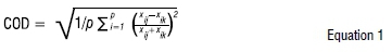
where x_ij and x_ik are the concentration for sampling interval i at sites j and k, respectively, and p is the number of sampling intervals. In terms of spatial distribution, a COD of 0 means that there are no differences between the observed concentrations at the two sites, while a value approaching 1 indicates that the two sampling sites are different.^53,55 Graphical analysis was also used in determining spatial variation. The inverse distance weighted (IDW) interpolation within the mapping software (ArcMap version 10.0) was applied to the annual and monthly concentrations of PM₁₀, PM_2.5 and the PM chemical components given that the number of sites was restricted by the cost. When data are sparse, the underlying assumptions about the variation among samples may differ and the use of a spatial interpolation method and parameters may become critical.^56,57 The performance of the spatial interpolation method is better when the sample density is higher.^58-60 However, the accuracy of regression modelling is not really dependent on the sampling density, but rather on how well the data are sampled and how significant the correlation is between the primary variable and secondary variable(s).⁶¹ To predict a value for any unmeasured location, IDW uses the measured values surrounding the prediction location. The measured values closest to the prediction location have a greater influence on the predicted value than those farther away. IDW assumes that each measured point has a local influence that diminishes with distance. It gives greater weight to points closest to the prediction location, and the weight diminishes as a function of distance.⁶²

APP calculation

The Air Pollution Model (TAPM) was used in the calculation of parameters needed to determine the APP. The dynamic parameters that were calculated included the MO length, wind velocity, planetary boundary layer height and turbulence parameters. The APP was determined according to the method of Swart⁶³ using Equation 2:

where P(APP) is the air pollution potential index, P(||) is the wind speed, P(H) is the planetary boundary layer and P(L) is the atmospheric stability. The APP index for a specific area can be classified as being favourable, moderate or unfavourable depending on the conditions set out for the parameters that are the driving force behind the APP calculation, as shown in Table 1.

 

 

In this study, APP, MO, MH and VC values were calculated and correlated with the PM measurement values collected during the sampling campaign.

 

Results and discussion

Figure 2 shows the annual concentrations of PM₁₀, PM_2.5 and PM chemical components. The annual concentrations of PM₁₀ were 38.11 µg/cm³ at Site 3, 31.28 µg/cm³ at Site 2, 31.02 µg/cm³ at Site 1, 24.65 µg/cm³ at Site 5, 24.10 µg/cm^{3 at Site 4}, and 20.98 µg/cm³ at Site 6. Annual PM₁₀ concentrations were below the South African National Ambient Air Quality Standard of 40 µg/cm³. The PM_2.5 concentrations are on average lower than the concentrations of SiAl-rich and SiAlFe-rich particles. This finding can be attributed to the fact that some PM_2.5 particles may have evaporated during the 3-5 week period during which the samplers were deployed in the field. The Fe-rich particles were the least abundant, with an annual average below 1 µg/cm³ across all sites. The C-rich particles had the same signature as PM_2.5, with the lowest concentration being around Site 6. The highest concentrations for Ca-rich particles were observed around sampling Site 6 which is located about 1.6 km west-northwest of Marula Platinum Mine, with the lowest concentrations around Site 4 and Site 5. The highest Si-rich, SiMg-rich, SiAl-rich and SiAlFe-rich particle concentrations were observed around sampling Site 3 which is about 1.7 km from the Samancor chrome smelter and 1.9 km from the silicone mine, with the lowest concentrations being observed at Site 6. The highest observed concentrations for FeCr-rich particles were at sampling Sites 3 and 5, and Site 5 is about 2 km from the ASA chrome smelter. The Cr-rich particles were highest at Site 1 and Site 3; Site 1 is about 2.5 km from the Glencore chrome smelter. The annual concentrations of Cr-rich particles across all the sites were above the 0.11 µg/m³ annual limit set by the New Zealand Ministry of Environment.⁶⁴ The highest PM₁₀ concentrations were measured during the winter months (May-July) except at Site 6 (Mashegoane) where the highest concentrations were observed during the month of November when there was soil tillage in preparation for crop sowing just before the rainy season. SiAl-rich and SiAlFe-rich particles were the most abundant particles with Fe-rich particles being less abundant. Si-rich, Cr-rich and CrFe-rich particles were more abundant closer to their sources.

Spatial variation

The annual spatial concentration map was generated using geographic information system software (Figure 3). The number of sampling sites was limited due to budgetary constraints, so IDW was used because it does not require a threshold for number of points. The choice of the IDW statistical method proved to be useful as it was able to predict the spatial variation of PM₁₀, PM_2.5 and PM chemical components in the study area. This output is very important for cash-strapped local authorities that are tasked with the responsibility of managing air quality in their jurisdiction because they can perform this analysis with limited resources. The maps in Figure 3 indicate that there is a distinct spatial heterogeneity in the study area with variability in both low and elevated concentrations being observed at different sites for PM₁₀, PM_2.5 and PM chemical components. This difference can be attributed to the vast distribution of sources in the area. The highest concentrations for annual PM₁₀, Cr-rich, Fe-rich, Si-rich, SiAl-rich, SiAlFe-rich and SiMg-rich particles were observed around Site 3, which is about 1.7 km from the Samancor chrome smelter and 1.9 km from the Silicone mine, which are located south-southeasterly of the sampling site. The highest Fe-rich, Si-rich and SiMg-rich concentrations were sparsely distributed. Lowest concentrations for the same particles were observed around Site 6. The highest concentrations for PM_2.5 and C-rich particles were observed around Site 1, and they have similar distribution patterns. The lowest concentrations of PM₁₀, PM_2.5 and PM chemical components were observed around Site 6, extending to Site 5 and Site 4. The only exception was SiAlFe-rich particles for which the lowest concentrations were observed to the northeast (Site 6) and southeast (Site 1) of the study area. FeCr-rich particles showed highest concentrations closer to the smelters around Site 3 and Site 5.

The highest Ca-rich concentrations were observed around Site 6, which is located in an area with black cotton soil. However, because the sites were not equally spaced in the study area, other methods such as the COD and r were used to confirm and validate the results of the spatial analysis determined using the geographic information system.

The COD values were calculated (Table 2) to characterise the spatial heterogeneity of PM₁₀, PM_2.5 and PM chemical components.

 

 

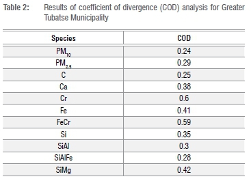
COD values higher than 0.2 indicate spatial heterogeneity, while COD values less than 0.1 indicate homogeneity of concentrations. All components in the study area had COD values greater than 0.2, which is an indication that there was a heterogeneous relation observed between the sites in the study area, and is in agreement with the observations in Figure 3. The lowest heterogeneity values for COD ranged from 0.24 to 0.4 and were observed for PM₁₀ (0.24), C-rich (0.25), SiAlFe-rich (0.28), PM_2.5 (0.29), SiAl-rich (0.3), Si-rich (0.35) and Ca-rich (0.38) particles. The moderate to highest COD values were observed for Fe-rich (0.41), SiMg-rich (0.42), FeCr-rich (0.59) and Cr-rich (0.6) particles. The highest COD values were observed for sites located in the vicinity of point source emitters, which indicates that the communities residing in the vicinity of these point sources are more vulnerable to the exposure of these particles than those living further downwind.

Influence of APP, MO, MH and VC on the distribution of PM₁₀

The annual influence of APP, MH, MO and VC on the distribution of PM₁₀ concentrations is shown in Figure 4a-d. The highest annual PM₁₀ concentrations are centred on Site 3 and distributed more to the east of the sampling site. The highest values for APP (Figure 4a) are centred to the south of the study area around Site 1, which is in contrast to the high APP values which are an indication of low dilution and poor dispersion of concentrations. The distribution of high concentrations to the east of Site 3 suggests that these concentrations move over the mountain slope to the east of Site 3, which is an indication that mountain winds may be responsible for this flow pattern. The lowest concentrations are centred on Site 6 and extend to Site 5 and Site 4. The lowest APP values are also encountered in the same area as that of the low PM₁₀ concentrations which is in contrast to the APP definition. Site 1 and Site 2 have moderate PM₁₀ concentrations, which could be attributed to the fact that the area from Site 4 to Site 6 is withina broader mountain valley floor base, compared to the area from Site 1 to Site 3 which has a narrow mountain valley floor base.

Figure 4b shows the comparison between PM₁₀ and MH. There is no correlation between PM₁₀ and MH. The highest MH was observed to the northeast of Site 3 which is supposed to be an area of low PM₁₀ concentrations; however, high PM₁₀ concentrations were observed in this region of high MH. The lowest PM₁₀ concentrations were observed where there was generally low MH, which is in contrast to the notion that low MH values are associated with poor dilution and dispersion resulting in accumulation of pollutants.

The relationship between PM₁₀ and MO is shown in Figure 4c. The area indicated by light green is an area with MO values below 0 and indicates favourable conditions for pollution dispersion. However, the lowest PM₁₀ concentrations were observed in an area with moderate stability values, with high PM₁₀ concentrations observed in an area of moderate MO. Therefore, MO was unable to correctly indicate the locations of high and low PM₁₀ concentrations. This anomaly between PM₁₀ concentrations and MO in a complex terrain is because MO is dependent on horizontal wind flows and local equilibrium.^39,65 However, these conditions do not hold in a complex terrain.³⁹ The MO was derived from synoptic circulations and showed stable conditions in areas where high and low PM₁₀ concentrations were observed. The model's inability to account for discontinuities in steep terrain suggests that the PM₁₀ concentrations within the valley floor were influenced by the thermal circulations within the valley, with upslope winds due to thermal heating favouring low PM₁₀ concentrations and downwind flows due to thermal cooling leading to stagnation and a possible increase in PM₁₀ concentrations. However, this hypothesis needs to be further tested in future studies with continuous ambient monitoring in the GTM.

Figure 4d shows the relationship between PM₁₀ and the VC. The VC shows moderate to high values to the west of the study area with moderate to low values spreading to the east of the study area. The highest VC values are observed around Site 6 with moderate values across all sites and low values observed to the northeast of Site 6. The observations show that there is a slight correlation between low PM₁₀ concentrations and high VC values, and poor correlation between high PM₁₀ concentrations and VC values.

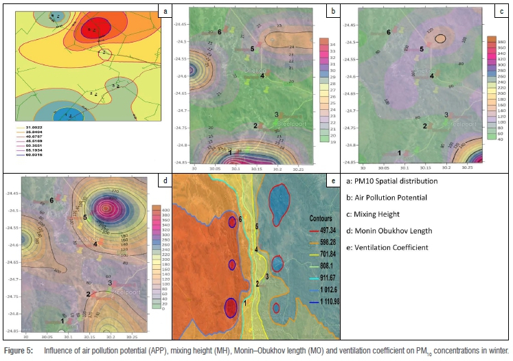
The seasonal influence of APP, MH, MO and VC on the distribution of PM₁₀ concentrations is shown in Figure 5 and Figure 6, for winter and summer, respectively. The highest PM₁₀ concentrations during the winter month of July were observed around sampling Site 5 which is located to the northeast of ASA chrome smelter. The lowest PM₁₀ concentrations were observed around Site 1 and Site 6, with moderate concentrations distributed across Site 2, Site 3 and Site 4. The highest APP values were concentrated around Site 1. Moderate APP values were observed to the northeast of Site 5 which is where high PM₁₀ concentrations were observed, and to the east of the study area. Low APP values were observed in areas with moderate PM₁₀ concentrations. The winter APP was unable to clearly identify areas with high and low PM₁₀ concentrations. The highest winter MH was observed to the southeast of the study area with moderate values spreading from southwest to northeast of Site 5. All other sites are located in regions with low MH, which is in contrast to the expected relation between MH and the expected dispersion ability of the atmosphere. The most favourable areas (MO≤0) for the dispersion of pollutants are indicated in Figures 5 and 6 by light green around Site 1 and Site 2. These areas are where the lowest PM₁₀ concentrations were observed. The most stable MO values were spatially distributed across Site 2, Site 3 and Site 4, which are areas where the highest pollution was expected. However, the highest concentrations were observed in an area of moderate MO values. This finding is an indication that the MO cannot clearly identify areas of high PM₁₀ concentrations in winter. Strong ventilation (VC) was observed to the west of the mountain valley and weak ventilation to the east of the mountain valley with moderate VC observed within the valley floor. This indicates that the winds within the valley were decoupled from winds outside the valley, and as a result, the VC cannot adequately predict the dispersion of pollutants in the study area.

During the summer month of December (Figure 6), the highest PM₁₀ concentrations were distributed around Site 1 and lowest concentrations observed around Site 4, Site 5 and Site 6, with moderate concentrations observed around Site 2 and Site 3. The high APP was distributed around Site 1 with moderate values distributed across Site 2, Site 3 and Site 4, and lower values around Site 5 and Site 6. The PM₁₀ concentrations are in agreement with the observed APP for all sites except Site 4 which is supposed to lie within a similar APP to that of Site 5 and Site 6. High MH values were observed to the southeast of the study area with moderate values distributed across Site 2, Site 3, Site 5 and Site 6. The lowest MH values were observed across Site 1 and Site 4. The PM₁₀ concentration was therefore expected to be highest around Site 1 and Site 4 in accordance with the definition of MH, with moderate PM₁₀ expected across all other sites. However, only results from Site 1 were in agreement with the observed MH. The most favourable conditions (with respect to MO) for the dispersal of pollutants were observed around Site 1, with unfavourable conditions observed around Site 2 and Site 4, and moderate conditions around Site 3, Site 5 and Site 6. The lowest VC values were observed around Site 1 and the highest VC values were observed around Site 6, with moderate values distributed across the remaining sites. Therefore, the VC was able to predict the areas for high PM₁₀ concentrations (Site 1) and low PM₁₀ concentrations (Site 6). Site 1 and Site 6 are located in the valley openings with Site 1 being in an area with a narrow valley opening and Site 2 being in an area with a wide valley opening. The strength of the valley flows depends on the valley volume. Wind speeds are often larger near the valley head where valley volume is small and the pressure gradient is high relative to distance from ridge top to ridge top. Wind speed weakens near the valley opening where the valley volume is larger and the pressure gradient is low relative to the distance between ridge tops.⁶⁶ Therefore, wind erosion may have played a major role in the observed high PM₁₀ concentrations at Site 1 and, similarly, calm conditions may have been responsible for the observed low PM₁₀ concentrations at Site 6. However, the VC did not have the same influence on the other sites which are situated in the middle of the valley floor. The reason could be that the TAPM model inputs terrain following coordinate systems and was unable to account for discontinuities in the steep terrain of the study area.

 

Conclusion

The University of North Carolina passive samplers coupled with CCSEM_EDS were used to determine spatial heterogeneity of PM chemical components. The concentrations of PM_2.5, PM₁₀ and PM chemical components were spatially heterogeneous with high heterogeneity observed near the industrial sources for FeCr-rich and Cr-rich particles and Si-containing particles. The COD values also showed that the highest heterogeneity was observed near the industrial sources. Findings showed little or no correlation between PM₁₀ and the meteorological parameters MH, MO length, APP and COD.

The findings highlight a very important point: passive samplers can be used (particularly in developing world contexts) as a substitute to more expensive continuous samplers to determine the spatial variation of PMs and their chemical components for effective environmental planning. The IDW interpolation within the mapping software (ArcMap version 10.0) was able to predict the spatial variation of PM₁₀, PM_2.5 and PM chemical components that indicated the existence of different conditions within the air shed, and therefore this variation may require different control strategies to mitigate the impacts of pollution within the air shed. The second finding was that synoptic winds used by the TAMP model were unsuccessful in determining the influence of APP, MO, MH and VC on the distribution of PM₁₀ concentrations in a complex terrain. This finding clearly indicates that these parameters are dependent largely on winds generated by temperature changes and mountain slopes in mountainous terrain. However, the VC was able to predict the areas for high PM₁₀ concentrations at the valley openings where the VC is influenced by the impact of pressure gradient on the wind strength. Therefore, for future analysis of the behaviour of pollutants in a complex terrain, a network of meteorological station balloon soundings within the valley floor and adjacent slopes needs to be set up in order to capture the actual meteorological parameters that influence the behaviour of air pollution. The ambient air quality should be monitored continuously to verify the findings of this study.

 

Acknowledgements

C.Y.W. receives research funding support from the South African Medical Research Council and the National Research Foundation (South Africa). C.T. thanks the South African Weather Service for provision of resources, space and time for conducting this research.

Authors' contributions

C.T. conceptualised the study, collected the samples, performed the GIS analysis, interpreted the data, wrote the initial draft of the manuscript and the revised version of the manuscript. C.Y.W. provided critical feedback and helped to shape the manuscript.

 

References

1.Gautam S, Prusty BK, Patra AK. Pollution due to particulate matter from mining activities. Reciklaža i održivi razvoj. 2012;5:53-58. Available from: https://www.rsd.tfbor.bg.ac.rs/download/arhiva_radova/2012/6_SnehaGAUTAM_ST.pdf        [ Links ]

2.Seinfeld JH, Pandis SN. Atmospheric chemistry and physics from air pollution to climate change. New York: John Wiley and Sons; 1998.         [ Links ]

3.Khlystov A, edited by Wittig B, Davidson C. Quality assurance project plan for Pittsburgh Air Quality Study (PAQS) [document on the Internet]. c2001 [cited 2018 Jun 15]. Available from: https://www3.epa.gov/ttnamti1/files/ambient/super/pittqapp.pdf        [ Links ]

4.Quality of Urban Air Review Group (AQUARG). Airborne particulate matter in the United Kingdom. Third report of the Quality of Urban Air Review Group [document on the Internet]. c1996 [cited 2018 Jun 10]. Available from: https://uk-air.defra.gov.uk/assets/documents/reports/empire/quarg/quarg_11.pdf        [ Links ]

5.Pope CA, Dockery W. Health effects of fine particulate air pollution: Lines that connect. J Air Waste Manag Assoc. 2006;56:709-742. https://doi.org/10.1080/10473289.2006.10464485        [ Links ]

6.Brook RD, Rajagopalan S, Pope CA, Brook JR, Bhatnagar A, Diez-Roux AV, et al. Particulate matter air pollution and cardiovascular disease: An update to the scientific statement from the American Heart Association. Circulation. 2010;121(21):2331-2378. https://doi.org/10.1161/CIR.0b013e3181dbece1        [ Links ]

7.World Health Organization (WHO). Health effects of particulate matter: Policy implications for countries in eastern Europe: Policy implications for countries in eastern Europe, Caucasus and central Asia. Copenhagen: WHO; 2013. Available from: http://www.euro.who.int/__data/assets/pdf_file/0006/189051/Health-effects-of-particulate-matter-final-Eng.pdf        [ Links ]

8.Hinds WC. Aerosol technology, properties, behavior, and measurements of airborne particles. 2nd ed. New York: John Wiley and Sons; 1999.         [ Links ]

9.Shah MH, Shaheen N, Jaffar M, Khalique A, Tariq SR, Manzoor S. Spatial variations in selected metal contents and particle size distribution in an urban and rural atmosphere of Islamabad, Pakistan. J Environ Manage. 2006;78:128-137. https://doi.org/10.1016/j.jenvman.2005.04.011        [ Links ]

10.Wang Y, Eliot MN, Koutrakis P, Gryparis A, Schwartz JD, Coull BA. Ambient air pollution and depressive symptoms in older adults: Results from the MOBILIZE Boston study. Environ Health Perspect. 2014;122(6):553-558. https://doi.org/10.1289/ehp.1205909        [ Links ]

11.Chan CK, Yao X. Air pollution in mega cities in China. Atmos Environ. 2008;42:1-42. https://doi.org/10.1016/j.atmosenv.2007.09.003        [ Links ]

12.Environmental Protection Agency (EPA). Technology Transfer Network (TTN). National air toxics assessments [webpage on the Internet]. c2010 [cited 2018 Jun 14]. Available from: https://www.epa.gov/national-air-toxics-assessment        [ Links ]

13.Ahrens CD. Meteorology today. 9th ed. Belmont, CA: Thomas Brooks/Cole; 2007. Available from: https://epdf.tips/meteorology-today-9th-edition.html        [ Links ]

14.Courault D, Drobinski P, Brunet Y, Lacarrere P, Talbot C. Impact of surface heterogeneity on a buoyancy-driven convective boundary layer in light winds. Bound Layer Meteorol. 2007;124:383-403. https://doi.org/10.1007/s10546-007-9172-y        [ Links ]

15.Reen BP, Stauffer DR, Davis KJ, Desai AR. A case study on the effects of heterogeneous soil moisture on mesoscale boundary layer structure in the southern Great Plains, USA. Part II: Mesoscale modelling. Bound Layer Meteorol. 2006;120:275-314. https://doi.org/10.1007/s10546-006-9056-6        [ Links ]

16.Yuan X, Xie Z, Zheng J, Tian X, Yang Z. Effects of water table dynamics on regional climate: A case 10 study over East Asian Monsoon Area. J Geophys Res. 2008;113, D21112, 16 pages. https://doi.org/10.1029/2008JD010180        [ Links ]

17.Yates DN, Chen F, Nagai H. Land surface heterogeneity in the Cooperative Atmosphere Surface Exchange Study (C 5 ASES-97). Part II: Analysis of spatial heterogeneity and its scaling. J Hydrometeorol. 2003;4:219-234. https://doi.org/10.1175/1525-7541(2003)4<219:LSHITC>2.0.CO;2        [ Links ]

18.Zhang N, Williams Q, Liu H. Effects of land-surface heterogeneity on numerical simulations of mesoscale atmospheric boundary layer processes. Theoret Appl Climatol. 2010;102:307-317. https://doi.org/10.1007/s00704-010-0268-9        [ Links ]

19.Atkinson BW. Mesoscale atmospheric circulation. London: Academic Press; 1981.         [ Links ]

20.Whiteman CD. Observations of thermally developed wind systems in mountainous terrain. In: Blumen W, editor. Atmospheric processes over complex terrain. Meteorological Monographs vol. 23. Boston, MA: American Meteorological Society; 1990. p. 5-42. https://doi.org/10.1007/978-1-935704-25-6_2        [ Links ]

21.Durran DR. Mountain waves and downslope winds. In: Blumen W, editor. Atmospheric processes over complex terrain. Meteorological Monographs vol. 23. Boston, MA: American Meteorological Society; 1990. p. 59-81. https://doi.org/10.1007/978-1-935704-25-6_4        [ Links ]

22.Whiteman CD, Doran JC. The relationship between overlying synoptic-scale flows and winds within a valley. J Appl Meteorol. 1993;32:1669-1682. https://doi.org/10.1175/1520-0450(1993)032<1669:TRBOSS>2.0.CO;2        [ Links ]

23.Wagner J, Leith D. Passive aerosol sampler. Part I: Principle of operation. Aerosol Sci Technol. 2001;34(2):186-192. https://doi.org/10.1080/027868201300034808        [ Links ]

24.Jiménez PA, González-Rouco JF, Montávez JP, Navarro E, García-Bustamante E, Valero F. Surface wind regionalization in complex terrain. J Appl Meteorol Climatol. 2007;47:308-324. https://doi.org/10.1175/2007JAMC1483.1        [ Links ]

25.Helgason W, Pomeroy JW. Characteristics of the near surface boundary layer within a mountain valley during winter. J Appl Meteorol Climatol. 2012;51:583-597. https://doi.org/10.1175/JAMC-D-11-058.1        [ Links ]

26.Geiger R. Das Klima der bodennahen Luftschicht. Ein Lehrbuch der Mikroklimatologie. 4. neubearbeitete und erweiterte Auflage mit 281 Abb., 646 S [The climate of ground-level air-layer. A textbook of microclimatology 4. New and expanded edition with 281 Abb.,646 S]. Brunswick: Verlag Friedrich Vieweg & Sohn; 1961. German. https://doi.org/10.1002/jpln.19620960108        [ Links ]

27.De Wekker SFJ, Kossmann M. Convective boundary layer heights over mountainous terrain: A review of concepts. Front Earth Sci. 2015;3(77):1-22. https://doi.org/10.3389/feart.2015.00077        [ Links ]

28.Zardi D, Whiteman D. Diurnal mountain wind systems. In: Chow F, De Wekker S, Snyder B, editors. Mountain weather research and forecasting: Recent progress and current challenges.: Dordrecht: Springer; 2013. p. 35-119. https://doi.org/10.1007/978-94-007-4098-3_2        [ Links ]

29.Bianco L, Djalaova IV, King CW, Wilczak JM. Diurnal evolution and annual variability of boundary-layer height and its correlation to other meteorological variables in California's Central Valley. Bound Layer Meteorol. 2011;140:491-511. https://doi.org/10.1007/s10546-011-9622-4        [ Links ]

30.Working Group 4 (WG4). COST 710: Pre-processing of meteorological data for dispersion models. Wind flow models over complex terrain for dispersion calculations [document on the Internet]. c1997 [cited 2018 Mar 11]. Available from: https://www2.dmu.dk/atmosphericenvironment/cost/docs/COST710-4.pdf        [ Links ]

31.Coulter RL. A comparison of three methods for measuring mixing-layer height. J Appl Meteorol. 1979;8:1495-1499. https://doi.org/10.1175/1520-0450(1979)018<1495:ACOTMF>2.0.CO;2        [ Links ]

32.Saurez MJ, Arakawa A, Randall DA. The parameterization of the planetary boundary layer in the UCLA general circulation model: Formulation and results. Mon Weather Rev. 1983;111:2224-2243. https://doi.org/10.1175/1520-0493(1983)111<2224:TPOTPB>2.0.CO;2        [ Links ]

33.Wesely ML, Cook DR, Hart RL, Speer RE. Measurements and parameterization of particulate sulfur dry deposition over grass. J Geophys Res. 1985;90:2131-2143. https://doi.org/10.1029/JD090iD01p02131        [ Links ]

34.Konor CS, Boezio GC, Mechoso CR, Arakawa A. Parametrization of PBL process in an atmospheric general circulation model: Description and preliminary assessment. Mon Weather Rev. 2009;37:1061-1082. https://doi.org/10.1175/2008MWR2464.1        [ Links ]

35.Rotach A, Gohm MN, Lang D, Leukauf I, Stiperski, Wagner JS. On the vertical exchange of heat, mass and momentum over complex, mountainous terrain. Front Earth Sci. 2015;3:76. Available from: https://www.frontiersin.org/articles/10.3389/feart.2015.00076/full        [ Links ]

36.Steyn DG, De Wekker SFJ, Kossmann M, Martilli A. Boundary layers and air quality in mountainous terrain. In: Chow FK, De Wekker SFJ, Snyder B, editors. Mountain weather research and forecasting: Recent progress and current challenges. Berlin: Springer; 2013. p. 261-289. https://doi.org/10.1007/978-94-007-4098-3_5        [ Links ]

37.Faiz A, Sinha K, Walsh M, Varma A. Automotive air pollution: Issues and options for developing countries. Washington DC: Infrastructure and Urban Development, World Bank; 1990. Available from: http://documents.worldbank.org/curated/en/743671468739209497/pdf/multi-page.pdf        [ Links ]

38.Figueroa-Esspinoza B, Salles P. Local Monin-Obukhov similarity in heterogeneous terrain. Atmos Sci Lett. 2014;15:299-306. https://doi.org/10.1002/asl2.503        [ Links ]

39.Grisogono B, Kraljevic L, Jericevic A. Notes and correspondence the low-level katabatic jet height versus Monin-Obukhov height. Q J R Meteorol Soc. 2007;133:2133-2136. https://doi.org/10.1002/qj.190        [ Links ]

40.Gross E. The National Air Pollution Potential Forecast Program: ESSA technical memorandum WBTM NMC 47 [document on the Internet]. c1970 [cited 2018 Mar 03]. Available from: https://apps.dtic.mil/dtic/tr/fulltext/u2/714568.pdf        [ Links ]

41.Iyer US, Raj P. Ventilation coefficient trends in the recent decades over four major Indian metropolitan cities. J Earth System Sci. 2013;122:537-549. https://doi.org/10.1007/s12040-013-0270-6        [ Links ]

42.Devara PCS, Raj PE. Lidar measurements of aerosols in the tropical atmosphere. Adv Atmos Sci. 1993;10:365-378. https://doi.org/10.1007/BF02658142        [ Links ]

43.Krishnan P, Kunhikrishnan PK. Temporal variations of ventilation coefficient at a tropical Indian station using UHF wind profiler. Curr Sci. 2004;86(3):447-451. Available from: https://www.currentscience.ac.in/Downloads/article_id_086_03_0447_0451_0.pdf        [ Links ]

44.Nath P, Patil RS. Climatological analysis to determine air pollution potential for different zones in India. In: Brebbia CA, Power H, Longhurst JWS, editors. Air pollution VIII [document on the Internet]. c2000 [cited 2018 Apr 15]. Available from: https://www.witpress.com/Secure/elibrary/papers/AIR00/AIR00048FU.pdf        [ Links ]

45.Anil Kumar KG. Air pollution climatology of Cochin for pollution management and abatement planning. Mausam. 1999;50:383-390. Available from: http://metnet.imd.gov.in/mausamdocs/15046.pdf        [ Links ]

46.Schulze BR. Climate of South Africa. Part 8: General survey WB28. Pretoria: SA Weather Bureau; 1986.         [ Links ]

47.South African Department of Water Affairs and Forestry (DWAF). Water Services Planning Reference Framework, Sekhukhune District Municipality [document on the Internet]. c2005 [cited 2018 Jun 13]. Available from: http://www.sekhukhunedistrict.gov.za/sdm-admin/documents/Sekhukhune%202011-12%20IDP.pdf        [ Links ]

48.Goovaerts P. Kriging vs stochastic simulation for risk analysis in soil contamination. In: Soares A, Gomez-Hernandez J, Froidevaux R, editors. geo-ENV I - Geostatistics for environmental applications. Dordrecht: Kluwer Academic Publishers; 1997. p. 247-258. https://doi.org/10.1007/978-94-017-1675-8_21        [ Links ]

49.Van Groenigen JW, Stein A, Zuurbier R. Optimization of environmental sampling using interactive GIS. Soil Tech. 1997;10:83-97. https://doi.org/10.1016/S0933-3630(96)00122-5        [ Links ]

50.Fraczek W, Bytnerowicz A, Legge A. Optimizing a monitoring network for assessing ambient air quality in the Athabasca oil sands region of Alberta, Canada. Alpine Space - Man Environ. 2009;48:127-142. Available from: https://www.researchgate.net/publication/313609727_Optimizing_a_monitoring_network_for_assessing_ambient_air_quality_in_the_Athabasca_oil_sands_region_of_Alberta_Canada        [ Links ]

51.Ott DK, Cyrs W, Peters TM. Passive measurement of coarse particulate matter, PM10-2.5. J Aerosol Sci. 2008;39(2):156-167. https://doi.org/10.1016/j.jaerosci.2007.11.002        [ Links ]

52.Sawvel EJ, Willis R, West RR, Casuccio GS, Norris G, Kumar N, et al. Passive sampling to capture the spatial variability of coarse particles by composition in Cleveland, OH. Atmos Environ. 2015;105:61-69. https://doi.org/10.1016/j.atmosenv.2015.01.030        [ Links ]

53.Lagudu URK, Raja S, Hopke PK, Chalupa DC, Utell MJ, Casuccio G, et al. Heterogeneity of coarse particles in an urban area. Environ Sci Technol. 2011;45:3288-3296. https://doi.org/10.1021/es103831w        [ Links ]

54.Hopke PK, Casuccio G. Scanning electron microscopy. In: Receptor modeling for air quality management vol. 7. Amsterdam: Elsevier; 1991; p. 149-212. https://doi.org/10.1016/S0922-3487(08)70129-1        [ Links ]

55.Wongphatarakul V, Friedlander SK, Pinto JP. A comparative study of PM_2.5 ambient aerosol chemical databases. Environ Sci Technol. 1998;32:3926-3934. https://doi.org/10.1021/es9800582        [ Links ]

56.Burrough PA, McDonnell RA. Principles of Geographical Information Systems. New York: Oxford; 1998.         [ Links ]

57.Hartkamp AD, White JW, Hoogenboom G. Interfacing GIS with agronomic modeling: A review. Agron J. 1999;91:917-928. https://doi.org/10.2134/agronj1999.915761x        [ Links ]

58.Webber D, Englund E. Evaluation and comparison of spatial interpolators. Math Geol. 1992;24(4):381-391. https://doi.org/10.1007/BF00891270        [ Links ]

59.Isaaks H, Srivastava MR. An introduction to applied geostatistics. New York: Oxford University Press; 1989. p. 561. Available from: https://www.scribd.com/document/266290280/An-Introduction-to-Applied-GEOostatistics-Isaaks-and-Srivastava-1989-Oxford        [ Links ]

60.Stahl K, Moore RD, Floyer JA, Asplin MG, McKendry IG. Comparison of approaches for spatial interpolation of daily air temperature in a large region with complex topography and highly variable station density. Agric Forest Meteorol. 2006;139:224-236. https://doi.org/10.1016/j.agrformet.2006.07.004        [ Links ]

61.Hengl T. A practical guide to geostatistical mapping of environmental variables. EUR 229404 EN. Luxembourg: Office for Official Publications of the European Communities; 2007. Available from: https://www.lu.lv/materiali/biblioteka/es/pilnieteksti/vide/A%20Practical%20Guide%20to%20Geostatistical%20Mapping%20of%20Environmental%20Variables.pdf        [ Links ]

62.Li L, Losser T, Yorke C, Piltner R. Fast inverse distance weighting-based spatiotemporal interpolation: A web-based application of interpolating daily fine particulate matter PM_2.5 in the contiguous U.S. using parallel programming and k-d tree. Int J Environ Res Public Health. 2004;11:9101-9141. https://doi.org/10.3390/ijerph110909101        [ Links ]

63.Swart A. An analysis of the air dispersion potential over Uubvlei, Oranjemund, Namibia [dissertation]. Pretoria: University of Pretoria; 2015. Available from: https://repository.up.ac.za/bitstream/handle/2263/60862/Swart_Assessment_2017.pdf?sequence=1&isAllowed=y        [ Links ]

64.Fisher G, Metcalfe J. Good practice guide for assessing discharges to air from industry. Wellington: NZ Ministry for the Environment; 2016. https://doi.org/10.13140/RG.2.1.3803.4162        [ Links ]

65.Monin AS, Obukhov AM. Basic laws of turbulent mixing in the surface layer of the atmosphere [translation]. Tr Akad Nauk SSSR Geophiz Inst. 1954;24(151):163-187. Available from: https://mcnaughty.com/keith/papers/Monin_and_Obukhov_1954.pdf        [ Links ]

66.Whiteman CD. Mountain meteorology: Fundamentals and applications. New York: Oxford University Press; 2000. p. 355. Available from: https://www.amazon.com/Mountain-Meteorology-Fundamentals-David-Whiteman/dp/0195132718#reader_0195132718        [ Links ]

 

 

Correspondence:
Cheledi Tshehla
Cheledi.Tshehla@weathersa.co.za

Received: 28 Mar. 2019
Revised: 14 May 2019
Accepted: 05 June 2019
Published: 26 Sep. 2019

 

 

EDITOR: Priscilla Baker
FUNDING: None