RESEARCH ARTICLES

 

An empirical investigation of alternative semi-supervised segmentation methodologies

 

 

Douw G. Breed; Tanja Verster

Centre for Business Mathematics and Informatics, North-West University, Potchefstroom, South Africa

Correspondence

 

 

---

ABSTRACT

Segmentation of data for the purpose of enhancing predictive modelling is a well-established practice in the banking industry. Unsupervised and supervised approaches are the two main types of segmentation and examples of improved performance of predictive models exist for both approaches. However, both focus on a single aspect - either target separation or independent variable distribution - and combining them may deliver better results. This combination approach is called semi-supervised segmentation. Our objective was to explore four new semi-supervised segmentation techniques that may offer alternative strengths. We applied these techniques to six data sets from different domains, and compared the model performance achieved. The original semi-supervised segmentation technique was the best for two of the data sets (as measured by the improvement in validation set Gini), but others outperformed for the other four data sets.
Significance:
•We propose four newly developed semi-supervised segmentation techniques that can be used as additional tools for segmenting data before fitting a logistic regression.
•In all comparisons, using semi-supervised segmentation before fitting a logistic regression improved the modelling performance (as measured by the Gini coefficient on the validation data set) compared to using unsegmented logistic regression

Keywords: data mining; predictive models; multivariate statistics; pattern recognition

---

 

 

Introduction

The use of segmentation within a predictive modelling context is a well-established practice in credit scoring.^1-3 According to Thomas³, its goal is to achieve more accurate, robust and transparent predictive models that allow lenders to better serve the segments identified. The origins of segmentation lie in marketing survey analysis, with the first application by Belson⁴ when studying the effects of BBC broadcasts in England. (For more information on the history of segmentation refer to Morgan et al.⁵) The only early approach still in broad use today is chi-squared automatic interaction detection⁶, which was developed initially by Kass⁷.

Predictive modelling refers to the use of statistical methods to construct formulae to estimate a target variable based on various explanatory variables. For this paper the target variables are binary, i.e. there are only two outcomes. The basis for model comparison is 'lift', i.e. the ability of the models to distinguish between the two outcomes compared to a naïve estimate.¹⁷ There are several ways to measure lift, and for this paper the Gini coefficient was chosen.

In this paper, the focus is segmentation when developing predictive models, irrespective of the application - credit risk, marketing, financial risk management, fraud detection, process monitoring, health and medicine, environmental analysis, etc. The results should therefore be of interest to researchers in any scientific or other field in which such models are applied. More specifically, this paper increases the number of available segmentation techniques available by proposing four alternative semi-supervised segmentation techniques.

There are two main types of segmentation - supervised and unsupervised - and the former are favoured in predictive modelling. Supervised techniques are used to identify cases that act alike, i.e. where 'independent' predictors display similar predictive patterns relative to a 'dependent' target variable. Separate segments are required to address interactions in which predictive patterns change with the values of other predictors, especially when developing generalised linear models. Interactions are often related to the target's value, and the focus is typically on maximising target separation - or impurity - between segments.⁶ The most obvious examples are decision trees derived using recursive partitioning algorithms, which identify homogenous risk groups on the assumption that they will display the greatest interactions. This is not always the case.

By contrast, unsupervised segmentation⁸ identifies subjects that look alike, i.e. have variables with similar values. It maximises segments' dissimilarities based on a distance function, with no dependent variable (one does not need a target). The most obvious examples are cluster and factor analysis, most commonly used in marketing.

The choice between supervised and unsupervised segmentation depends on the application and requirements of the models developed⁹, and many examples of improved model performance exist for both¹⁰. However, both focus on a single aspect (i.e. act or look alike) and so using them together may deliver better results.

Their combined use considers both target and explanatory variables, and is called semi-supervised segmentation (SSS).^11-13 It has many similarities with semi-supervised clustering¹⁴, supervised clustering¹⁵ and semi-supervised semantic segmentation¹⁶ (more used in image processing). For more detail on the differences and similarities see Breed¹¹. In this paper, we explore four newly developed variations of an existing technique to see whether they can provide further benefits.

Six data sets were used from different disciplines, each of which was split into a training and validation set. The five different SSS approaches were applied to each to see which worked best, with models built per segment using logistic regression. A further model was developed on the unsegmented data. Of the five approaches, four are new alternatives and form the main contribution of this paper. They were inspired by an existing technique, semi-supervised segmentation using k-means clustering and information value (SSSKMIV), which was explored in Breed et al.¹³ and described in more detail in a recent PhD thesis¹¹. K-means clustering is used to measure the independent variable distribution, and information value for target separation. A 'supervised weight' controls the balance between the two aspects.¹³ The algorithm is quite complex and calculation intensive, so alternatives were sought. The four variations are:

Variation 1: We replaced the information value with the chi-squared test statistic and call this technique SSSKMCSQ (semi-supervised segmentation as applied to k-means using chi-squared). The chi-squared calculation has similarities with the Hosmer-Lemeshow statistic, and further information can be found in Hand⁶.

Variation 2: We developed a density-based semi-supervised technique using Wong's density-clustering algorithm.¹⁸ We call this the SSSWong technique (semi-supervised segmentation applied to Wong's density clustering methodology).

Variation 3: We developed a semi-supervised technique with segment size equality (SSE). We call this the SSSKMIV_SSE technique (semi-supervised segmentation applied to the k-means algorithm using information value as supervised component, with the addition of segment size equality).

Variation 4: These techniques (SSSKMIV, SSSKMCSQ, SSSKMIV_SSE) have some similarities with the k-means semi-supervised segmentation algorithm, proposed in Peralta et al.¹⁹ which is called LK-Means. This methodology has many similarities to SSS techniques, but also has a number of clear differences.¹¹ Our fourth variation augments other existing semi-supervised techniques¹¹ to make its results comparable to the others. It is thus not really new, but an existing supervised technique adapted to be comparable with other SSS techniques.

 

Semi-supervised techniques

Both unsupervised and supervised segmentation make intuitive sense depending on the application and the requirements of the models developed⁹ and many examples exist in which the use of either improved model performance¹⁰. However, both focus on a single aspect (i.e. either target separation or independent variable distribution) and using them in tandem might deliver better results. Five semi-supervised techniques are described here, four of which are new.

Semi-supervised segmentation: SSKMIV

This approach is explored in Breed et al.²⁰ and described in more detail in a recent PhD thesis¹¹ and will be used as the first (original) segmentation method. It is called SSSKMIV, an abbreviation for semi-supervised segmentation using k-means clustering and information values, where k-means is used to assess independent variable distributions, and information values for target separation.

The implementation of this approach is quite complex and calculation intensive.^11,20 Further, the information value formula demands that there be at least one event and non-event each time (to avoid division by zero), and results can be distorted by small numbers. A general rule is that each bin and segment combination must have at least five events and five non-events.

Semi-supervised segmentation: SSKMCSQ (Variation 1)

In this variation the information value is replaced with the chi-squared⁶ test statistic for the supervised part, and we call this SSSKMCSQ (semi-supervised segmentation as applied to k-means using chi-squared).

The chi-square statistic is often used as a measure of separation. A good example is chi-squared automatic interaction detection, which is a recursive partitioning algorithm used to construct decision trees.⁶ It is used here to compare observed target values for each segment against naïve estimates (i.e. counts per class proportional to those for the population).

Using the chi-squared for the supervised part has two main advantages:

•It is always defined within a segmentation scheme (no division by zero). Our techniques do have the option that a user can set a minimum number of cases. A popular rule of thumb is to have at least 5% of cases of the sample in each segment.²

•It works for both binary and continuous variables - which allows its application to a broader range of problems.

Details of the k-means clustering technique are provided below, followed by a formal definition of chi-squared.

Consider a data set with n observations and m characteristics and let x_i={x_i1,x_i2,...x_im} denote a single observation in the data set. The n x m matrix comprising all characteristics for all observations is denoted by X. Let X_p = {X_1p, X_2p,..., X_np} denote a vector of all observations for a specific characteristic p.

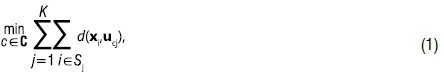
On completion of the k-means clustering algorithm all observations x_i, with i = {1,2,...,n}, will have been assigned to one of the segments S₁,S₂,...,S_K where each S_j denotes an index set containing the observation indices of all the variables assigned to it. That is, if observation x_i is assigned to segment S_j, then i∈S_j .

Further, let u_j = {u_j1,u_j2,...u_jm} denote the mean (centroid) of segment S_j, for example u_j1 will be the mean of characteristic X₁. The distance from each observation x_i to the segment mean u_j is given by a distance function d(x_i,u_j). If a Euclidian distance measure is used, then d(x_i,u_j)=||x_i-u_j||² where ||.||² defines the distance. Note that the double vertical bars indicate distance and hence imply that a square root is used.

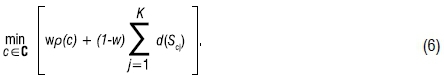
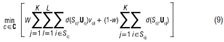
The objective of ordinary k-means clustering is to minimise within-segment distances. For notational purposes, we introduce c∈C as an index of an assignment of all the observations to different segments, with C the set of all combinations of possible assignments. The notation S_cj is now introduced to reference all the observations for a given assignment c∈C and for a given segment index j. In addition, u_cj is the centroid of segment S_cj. The objective function of the ordinary k-means clustering algorithm can now be stated in generic form as

Note that the notation used for the k-means clustering is the same notation as used in Breed et al.²⁰

For the newly proposed SSSKMCSQ technique, a function is required to inform the segmentation process. For the supervised component, we will use the chi-squared value (rather than the information value).

The chi-square statistic is calculated as

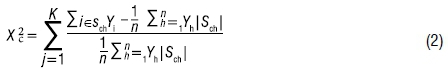
where n is the number of observations in the input data set; K is the number of segments over which is calculated; and y is the target variable and can be either binary or continuous. The term |S| is used to represent the number of observations in segment S.

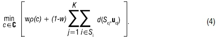
If chi-square is used in semi-supervised segmentation, then the supervised component ρ(c) for each observation x_i and segment S_cj (with i assigned to S_cj in each case) can be defined as

Let 0 ≤ w ≤ 1 be a weight that controls how much the clustering function is penalised by the chi-square statistic. The proposed optimisation problem for the SSSKMCSQ technique, taking within-segment distances into account, is the following

In this paper, a heuristic approach is followed for the purpose of generating solutions to the optimisation problem in [4]. This includes determining the optimal weight w for the supervised portion, using an algorithm that consists broadly of 10 steps similar to those of SSSKMIV. For details of the steps, see Breed et al.²⁰

Semi-supervised segmentation: SSSWong (Variation 2)

Next, we propose a density-based semi-supervised technique using Wong's density clustering algorithm.¹⁸ We call this the SSSWong technique (semi-supervised segmentation applied to Wong's density clustering methodology).

Predictive models are often developed for relatively large data sets (>1000 observations and 20 or more characteristics), and more common kernel-based density methods (like k-nearest neighbours²¹) are inviable because of their complexity. Wong's methodology combines the speed of k-means with the advantages of density-based clustering. It consists of two stages.^18,21 Note that these two stages are in essence an iterative process.

Stage 1: A preliminary clustering analysis is performed using a k-means algorithm with k much larger than the number of final clusters required.

Stage 2: The k-clusters formed in stage one are analysed and combined based on density-clustering dissimilarities until the required number of clusters are formed, or only a single cluster remains.

Preliminary clusters s_cr and s_ct are considered adjacent if the midpoint between the centroids u_cr and u_ct are closer to each other than any other preliminary-cluster mean based on Euclidean distance. Each thus has only one potential cluster with which it can be combined (with ties typically dealt with based on the order of the observations in the data set). The pair combined each time is that with the minimum density-based dissimilarity measure (see Wong¹⁸ for further detail and the derivation):

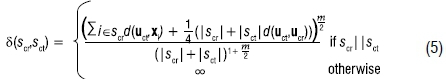
where |s| represents the number of observations in segment s and s_cr||s_ct indicates that s_cr is adjacent to s_ct.

Wong's clustering was incorporated in the original semi-supervised technique (SSKMIV). We adjusted Wong's second step to incorporate the target variable. Thus, the algorithm optimises both cluster density and target rate differences. Let c∈C denote an index of an assignment of all the preliminary segments s_c1,s_c2,...,s_cq to the final segments S_c1,S_c2,...,S_cK with K > q and with C the set of all combinations of possible assignments. In this case, q denotes the number of preliminary segments. Note that each will contain at least one observation, but is likely to contain a larger number that reduces computational complexity on large data sets.

The conglomeration of the preliminary segments into the final set of segments is done in a binary fashion, as illustrated by Figure 1.

 

 

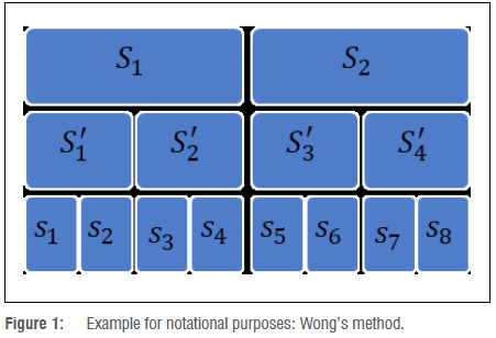
The final segments for the example are S1 = {S'₁,S'₂} = {s₁,s₂,s₃,s₄} and S₂= {S'₃,S'₄}={s₅,s₆,s₇,s₈}. This previous example covers only one possible combination of assignments. We use the notation S_cj to represent any set of segments assigned to it for a given combination c∈C. In order to evaluate the density dissimilarity between two segments or nodes, we make use of the notation d(S_cj). For example, to calculate the dissimilarity between nodes S'₁ and S'₂, we can calculate d(S'_c1)=d (s₁,s₂).

The proposed optimisation problem for the SSSWong algorithm is:

Note the values of ρ(c) and d(S_cj) are standardised for the same reasons as when using SSSKMIV.²⁰ For a single segmentation analysis using SSSWong, there are five steps:

1.Preliminary segmentation: Similar to Wong's method, the first step creates the preliminary segments that will be iteratively combined using formula [6].

2.Preliminary segment inspection: Preliminary segments are investigated to identify any with no events or non-events (which the information value calculation cannot handle), which are combined using Wong's standard density measure.

3.Determine preliminary segment adjacency: Adjacent segments are identified for each preliminary segment using a k-nearest neighbour type approach.

4.Combine segments until K left: Segments are iteratively combined until the required number of segments remains.

5.Calculate data set statistics: Statistics like information value obtained per segment are calculated and stored for further use.

The details of these steps can be found in Chapter 7 of a recent PhD thesis.¹¹

Semi-supervised segmentation: SSKMIV_SSE (Variation 3)

For the third variation we developed a semi-supervised technique with segment-size equality (SSE). We call this the SSSKMIV_SSE technique (semi-supervised segmentation applied to the k-means algorithm using information value as supervised component, with the addition of segment size equality). Its purpose is to discourage the formation of small segments, or rather encourage segments of similar (or more equal) size.

Only minor adjustments were needed to the SSSKMIV's objective function¹¹, by introducing v as the SSE weight and δ as the SSE function. We define δ as

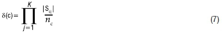
where n_c is the total number of assigned observations for c∈C. The function is at its maximum when all segment sizes (|S_c1|,...,| S_cK|) are equal. Incorporating v and δ into the SSSKMIV technique results in a new objective function:

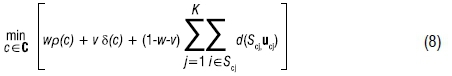
where w + v ≤ 1.

Semi-supervised segmentation: LK-Means (Variation 4)

The SSSKMIV variation has some similarities with the k-means semi-supervised segmentation algorithm, proposed in Peralta et al.¹⁹ which is called LK-Means. This methodology has many similarities to SSS algorithms, but also some clear differences.¹¹ For our fourth variation we augmented the LK-Means methodology. It is thus not really a new SSS technique, but an existing technique adapted to be comparable with others presented in this paper.

All four variations of semi-supervised segmentation methods (as well as the original SSSKMIV) were implemented in SAS software (Version 9.4, SAS Institute Inc., Cary, NC, USA). The detail of the technical specifications (e.g. the optimal number of segments, the weight parameters in SSS, the optimal value of k in the k-mean algorithm, and a heuristic example) can be found in Breed¹¹.

To facilitate representing the objective function of the LK-Means algorithm mathematically, we expand the S_cj notation to S_cjl, to reference all the observations for a given assignment c∈C, for a given segment index j and a given label l. Similarly, u_cjl represents the mean, or centroid of S_cjl. For this algorithm, the assumption is that the labels (or target variable values) take on L discrete values and are not continuous. The objective function of the LK-Means algorithm to be minimised becomes

where v_cjl is the ratio of the number of observations assigned to cluster j with label l divided by the number of total observations assigned to cluster j. This ratio represents the 'confidence' of label l in cluster j. The distortion weight, w, is similar to the weight in SSSKMIV and again adjusts the supervised element with values between 0 and 1. More details of these steps can be found in Chapter 7 of the PhD thesis.¹¹

 

How to measure model performance: Data splitting and Gini coefficient

In order to compare model performance, each data set was divided randomly into equally sized development and validation sets. Data splitting is the dividing of a sample into two parts and then developing a hypothesis using one part and testing it on the other.²² Picard and Berk²³ review it in the context of regression and provide specific guidelines for the validation of regression models, i.e. 25% to 50% of the data is recommended for validation. Faraway²⁴ illustrates that split-data analysis is preferred to a full-data analysis for predictions with some exceptions.

We used the development set (i.e. training data) to develop the predictive models, whilst the validation set (i.e. hold-out data) was used to assess model performance (hereafter the 'lift'). Lift was measured by calculating Gini coefficients², to quantify a model's ability to discriminate between two possible values of a binary target variable¹⁷. Cases are ranked according to the predictions, and the Gini then provides a measure of correctness. It is one of the most popular measures used in retail credit scoring^1-3,25, and has the added advantage that it is a single number¹⁷. For this paper, values are calculated for the combined validation data sets. Although we used only Gini in this paper, more measures were used in the original PhD thesis.¹¹

 

Description of data sets

The above segmentation techniques were compared on six different data sets, described below. All explanatory variables were standardised by transforming them into z-scores, i.e. subtracting the mean and dividing by the standard deviation of each based on the full development data set. Weights of evidence or dummy variables would have been preferable, but were not considered because of the added complexity of binning each predictor - especially if done per segment. We cannot say whether or how the transformation methodology might have affected the results.

The data sets are the same as those used in the previous study.¹² A short summary of the data used is given in Table 1. Details on the data sets can be found in Breed¹¹.

 

 

 

Empirical results

The five semi-supervised segmentation techniques described above were applied to all six data sets, with performance assessed on the validation data. Results for all five are presented in Tables 2-7, respectively, with Table 8 providing a summary of the results. Note that for a comparison of supervised and unsupervised techniques, please refer to other research studies.^11-13 Also, while our focus was to compare different semi-supervised segmentation techniques, we have also included an unsegmented logistic regression in each table as a further baseline.

 

 

 

 

 

 

 

 

 

 

 

 

 

 

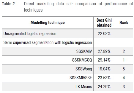
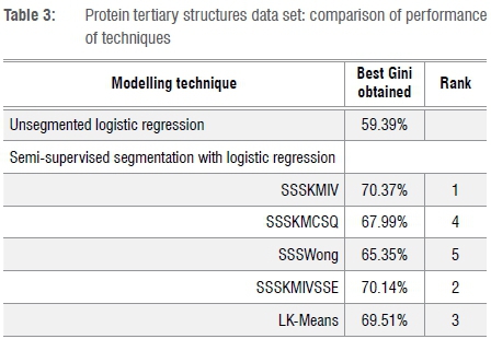
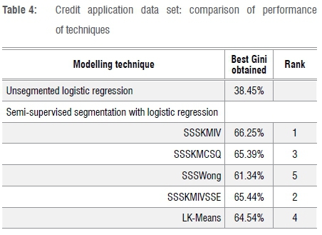
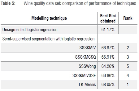
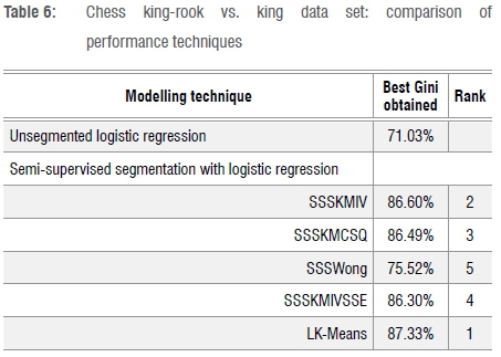
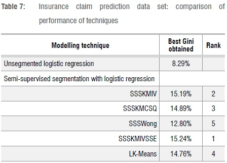
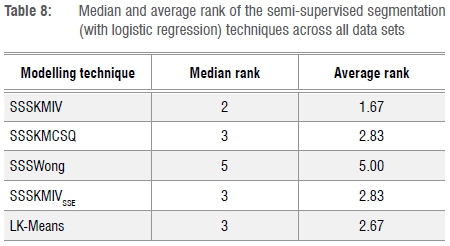
Table 2 summarises the performance of the modelling techniques when applied to the direct marketing data set (as measured by the Gini coefficient calculated on the validation set). SSSKMCSQ achieved the best result, with SSSKMIV second.

Table 3 summarises the results for the protein tertiary structures data set, where the ranking order is completely different from that in Table 2. As a start, SSSKMCSQ ranks fourth of five. Best is SSSKMIV, with SSSKMIV_SSE second. The Gini coefficients are between 65% and 70%, which are quite high values.

Table 4 shows results for the credit application data set, where SSSKMIV again outperforms the other techniques. Note that strong bureau data as well as internal data were available on this credit application data set, hence the relatively high Gini values. The large difference between the unsegmented and segmented results is highly unusual, and may be related to the use of z-scores (i.e. standardisation of variables). It may be that the variables that predict credit risk (delinquency) best, are the least normally distributed.

For the wine quality data set, Table 5 shows that one of our new variations takes top position: LK-Means.

Table 6 shows results for the chess king-rook vs. king data set, where LK-Means again dominates. It is interesting that the Gini coefficients achieved are very high, from 75% to almost 88%. It seems that it is easier to obtain efficient ranking in this data set, which relates to a highly structured game.

Table 7 shows the results for the last data set, which is for insurance claim prediction. In this case, SSSKMIV_SSE works best. The Gini coefficients are very low (Gini ranging between 12% and 16%), which makes one wonder about whether predictive models can provide any value in this domain.

And finally, Table 8 provides a summary of the median and average ranks for all five semi-supervised segmentation techniques.

The original SSSKMIV technique performed best with a median rank of 2 and average of 1.67. Three of the four variations (SSSKMCSQ, SSSKMIV_SSE, LK-Means) achieved a median rank of 3, while LK-Means achieved an average rank of 2.67 (only slightly higher than SSSKMCSQ and SSSKMIV_SSE). The overall loser was SSSWong, which came in last across the board.

Comments on using Gini as an absolute value

The analysis above illustrates the problem of using Gini as an absolute value.²⁷ The best was 87.33% for LK-Means on the chess data set, but for the insurance data the best was SSSKMIV_SSE with a Gini of 15.24%. Such results are not a reflection of the techniques being used, but the data under consideration.³³ It is unreasonable to have a minimum Gini that is broadly applied.³⁴ Using Gini coefficients for comparison makes sense only if the data are comparable - in this instance different models applied to the same data.

 

Concluding remarks

We proposed four newly developed semi-supervised segmentation techniques and provided their mathematical notation. Additionally, we evaluated our four variations against the original semi-supervised technique, SSSKMIV, on six different data sets, with Gini coefficients derived using combined validation data for each segment. The original SSSKMIV technique performed best overall and was the outright winner for two of the data sets, but other variations dominated elsewhere. Best performers were SSSKMIV in the protein and credit data sets, LK-Means in the wine quality and chess data sets, SSSKMIV_SSE in the insurance prediction data set and SSSKMCSQ in the direct marketing data set. The SSSWong technique produced the worst overall results, perhaps because some of k-means' weaknesses were already addressed by SSSKMIV¹¹ and the additional complexity of SSSWong adds no additional benefit.

We conclude that the four alternatives provide additional tools for segmenting data before fitting a logistic regression. Of the four, SSSWong is quickest to perform on a standard PC, but performs worst (as per the results observed). SSSKMCSQ is most versatile (as it can be performed on both binary and continuous variables) and achieves reasonable results. The most optimal variation will, however, be dependent on the characteristics of the data set being analysed.

The benefit of segmentation was also clearly illustrated in the six data sets used in previous work,¹² although the impact of the transformation methodology is not known. In this study, we have also clearly highlighted the danger of using an absolute Gini coefficient to evaluate the performance of any predictive model. The relative Gini value is more appropriate. Future research could include investigating which properties of data sets contribute to the differences in performance between the techniques. Another extension of the research could be to use measures other than Gini and information value; many other measures exist that could be alternatives to these values. Further comparisons could be done using an array of such alternative measures. It would also provide value to investigate transformation methodologies other than the z-score when doing such research.

 

Acknowledgements

We gratefully acknowledge the valuable input given by the anonymous referees. This work is based on research supported in part by the Department of Science and Technology (DST) of South Africa. The opinions, findings and conclusions or recommendations expressed in this publication are our own and the DST accepts no liability whatsoever in this regard.

 

Authors' contributions

D.G.B. was responsible for conceptualisation; methodology; data collection; data analysis; validation; data curation; writing revisions. T.V. was responsible for conceptualisation; sample analysis; data analysis; writing the initial draft; revisions; student supervision; project leadership and project management.

 

References

1.Anderson R. The credit scoring toolkit: Theory and practice for retail credit risk management and decision automation. New York: Oxford University Press; 2007.         [ Links ]

2.Siddiqi N. Credit risk scorecards. Hoboken, NJ: John Wiley & Sons; 2006.         [ Links ]

3.Thomas LC. Consumer credit models. New York: Oxford University Press; 2009. http://dx.doi.org/10.1093/acprof:oso/9780199232130.001.1        [ Links ]

4.Belson W. Effects of television on the interests and initiative of adult viewers in greater London. Br J Psychol. 1959;50(2):145-158. https://doi.org/10.1111/j.2044-8295.1959.tb00692.x        [ Links ]

5.Morgan JN, Solenberger PW, Nagara PR. History and future of binary segmentation programs. University of Michigan: Survey Research Center, Institute for Social Research; 2015. Available from: http://www.isr.umich.edu/src/smp/search/search_paper.html        [ Links ]

6.Hand DJ. Construction and assessment of classification rules. West Sussex: John Wiley & Sons; 1997.         [ Links ]

7.Kass GV. An exploratory technique for investigating large quantities of categorical data. J R Stat Soc Ser C Appl Stat. 1980;29(2):119-127. https://doi.org/10.2307/2986296        [ Links ]

8.Friedman J, Hastie T, Tibshirani R. The elements of statistical learning. Berlin: Springer; 2001. https://doi.org/10.1007/978-0-387-21606-5_14        [ Links ]

9.Cross G. Understanding your customer: Segmentation techniques for gaining customer insight and predicting risk in the telecom industry. Proceedings of the SAS Global Forum 2008; 2008 March 16-19. Cary, NC: SAS Institute Inc.; 2008. Paper 154-2008. Available from: http://www2.sas.com/proceedings/forum2008/154-2008.pdf        [ Links ]

10.Fico. Using segmented models for better decisions [document on the Internet]. c2014 [cited 2015 Jan 05]. Available from: http://www.fico.com/en/node/8140?file=9737        [ Links ]

11.Breed DG. Semi-supervised segmentation within a predictive modelling context [PhD thesis]. Potchefstroom: North-West University; 2017.         [ Links ]

12.Breed DG, Verster T. The benefits of segmentation: Evidence from a South African bank and other studies. S Afr J Sci. 2017;113(9/10), Art. #2016-0345, 7 pages. http://dx.doi.org/10.17159/sajs.2017/20160345        [ Links ]

13.Breed DG, De La Rey T, Terblanche SE. The use of different clustering algorithms and distortion functions in semi supervised segmentation. In: Proceedings of the 42nd Operations Research Society of South Africa Annual Conference; 2013 September 15-18; Stellenbosch, South Africa. Available from: http://www.orssa.org.za/wiki/uploads/Conf/ORSSA2013_Proceedings.pdf        [ Links ]

14.Grira N, Crucianu M, Boujemaa N. Unsupervised and semi-supervised clustering: A brief survey. In: A review of machine learning techniques for processing multimedia content: Report of the MUSCLE European Network of Excellence [document on the Internet]. c2005 [cited 2018 Jan 08]. Available from: http://cedric.cnam.fr/~crucianm/src/BriefSurveyClustering.pdf        [ Links ]

15.Eick CF, Zeidat N, Zhao Z. Supervised clustering algorithms and benefits. In: Proceedings of the 16th IEEE International Conference on Tools with Artificial Intelligence (ICTAI04); 2004 November 14-17; Boca Raton, FL, USA. Washington DC: IEEE; 2004. p. 774-776. http://dx.doi.org/10.1109/ICTAI.2004.111        [ Links ]

16.Hung WC, Tsai YH, Liou YT, Lin YY, Yang MH. Adversarial learning for semi-supervised semantic segmentation. CoRR (Computer Vision and Pattern Recognition) [preprint]. arXiv 2018; #1802.07934. Available from: http://arxiv.org/abs/1802.07934        [ Links ]

17.Tevet D. Exploring model lift: Is your model worth implementing? Actuarial Rev. 2013;40(2):10-13.         [ Links ]

18.Wong MA. A hybrid clustering method for identifying high-density clusters. J Am Stat Assoc. 1982;77(380):841-847. http://dx.doi.org/10.2307/2287316        [ Links ]

19.Peralta B, Espinace P, Soto A. Enhancing K-Means using class labels. Intell Data Anal. 2013;17(6):1023-1039. http://dx.doi.org/10.3233/IDA-130618        [ Links ]

20.Breed DG, Verster T, Terblanche SE. Developing a semi-supervised segmentation algorithm as applied to k-means using information value. ORION. 2017;33(2):85-103. http://dx.doi.org/10.5784/33-2-568        [ Links ]

21.Wong MA, Lane T. A kth nearest neighbour clustering procedure. In: Eddy WF, editor. Computer Science and Statistics: Proceedings of the 13th Symposium on the Interface. New York: Springer; 1981. https://doi.org/10.1007/978-1-4613-9464-8_46        [ Links ]

22.Barnard GA. Discussion of cross-validatory choice and assessment of statistical predictions. In: Stone M. Cross-validatory choice of statistical predictions. J R Stat Soc Ser B Stat Methodol. 1974;36:111-135.         [ Links ]

23.Picard P, Berk K. Data splitting. Am Stat. 1990;44(2):140-147. http://dx.doi.org/10.1080/00031305.1990.10475704        [ Links ]

24.Faraway JJ. Does data splitting improve prediction. Stat Comput. 2016;26:49-60. http://dx.doi.org/10.1007/s11222-014-9522-9        [ Links ]

25.Baesens B, Roesch D, Scheule H. Credit risk analytics: measurement techniques, applications, and examples in SAS. Hoboken, NJ: Wiley; 2016.         [ Links ]

26.Lichman M. Physicochemical properties of protein tertiary structure [data set on the Internet]. In: UCI Machine Learning Repository. c2013 [cited 2016 May 06]. Available from: http://archive.ics.uci.edu/ml        [ Links ]

27.Protein Structure Prediction Center [homepage on the Internet]. c2015 [cited 2016 Jun 04]. Available from: http://predictioncenter.org/        [ Links ]

28.Kaggle [homepage on the Internet]. c2016 [cited 2016 Sep 23]. Available from: http://www.kaggle.com        [ Links ]

29.Cortez P, Cerdeira A, Almeida F, Matos T, Reis J. Modeling wine preferences by data mining from physicochemical properties. Decis Support Syst. 2009;47(4):547-553. http://dx.doi.org/10.1016/j.dss.2009.05.016        [ Links ]

30.Casti JL, Casti JL. Five golden rules: Great theories of 20th-century mathematics and why they matter. New York: John Wiley & Sons; 1996.         [ Links ]

31.Russell SJ, Norvig P. Artificial Intelligence: A modern approach. 2nd ed. New Delhi: Pearson Education; 2003.         [ Links ]

32.Clarke M. A quantitative study of king and pawn against king. In: Clarke MRB, editor. Advances in computer chess. Edinburgh: Edinburgh University Press; 1977. p. 108-118.         [ Links ]

33.Hamerle A, Rauhmeier R, Rösch D. Uses and misuses of measures for credit rating accuracy. Technical Paper from the University of Regensburg. c2003. [cited 2017 Jan 17]. Available from: http://mx.nthu.edu.tw/~jtyang/Teaching/Risk_management/Papers/Testing/Uses%20and%20Misuses%20of%20Measures%20for%20Credit%20Rating%20Accuracy.pdf        [ Links ]

34.Engelman B, Rauhmeier R. The Basel II risk parameters: Estimation, validation, and stress testing. 2nd ed. Berlin: Springer; 2011. https://doi.org/10.1007/978-3-642-16114-8        [ Links ]

 

 

Correspondence:
Tanja Verster
Tanja.Verster@nwu.ac.za

Received: 13 Aug. 2018
Revised: 11 Jan. 2019
Accepted: 14 Jan. 2019
Published: 27 Mar. 2019