


Services on Demand
Article
 English (pdf)
 Article in xml format
 Article references
Indicators

Related links
-
 Cited by Google
 -
 Similars in Google
Share

 Permalink
South African Journal of Science
On-line version ISSN 1996-7489
Print version ISSN 0038-2353
S. Afr. j. sci. vol.115 n.1-2 Pretoria Jan./Feb. 2019
http://dx.doi.org/10.17159/sajs.2019/5204
RESEARCH ARTICLE
Observations from SANSA's geomagnetic network during the Saint Patrick's Day storm of 17-18 March 2015
Emmanuel Nahayo; Pieter B. Kotzé; Pierre J. Cilliers; Stefan Lotz
South African National Space Agency (SANSA), Hermanus, South Africa
ABSTRACT
Geomagnetic storms are space weather events that result in a temporary disturbance of the earth's magnetosphere caused by a solar wind that interacts with the earth's magnetic field. We examined more closely how some southern African magnetic observatories responded to the Saint Patrick's Day storm using local K-indices. We show how this network of observatories may be utilised to model induced electric field, which is useful for the monitoring of geomagnetically induced anomalous currents capable of damaging power distribution infrastructure. We show an example of the correlation between a modelled induced electric field and measured geomagnetically induced currents in southern Africa. The data show that there are differences between global and local indices, which vary with the phases of the storm. We show the latitude dependence of geomagnetic activity and demonstrate that the direction of the variation is different for the X and Y components.
SIGNIFICANCE:
•The importance of ground-based data in space weather studies is demonstrated.
•We show how SANSA's geomagnetic network may be utilised to model induced electric field, which is useful for the monitoring of geomagnetically induced anomalous currents capable of damaging power distribution infrastructure
Keywords: geomagnetic variations; geomagnetic storms; geomagnetically induced currents
Introduction
Geomagnetic storms can affect communication satellites, interrupt radio communication by changing the status of the ionosphere, induce low frequency electric currents in long conductors like power lines and disrupt power grids. During a magnetic storm, magnetospheric currents are diverted through the earth's ionosphere causing large disturbances in the geomagnetic field observed on the ground. These rapid fluctuations in the ground magnetic field are also the source of induced electric fields in the earth's surface.1 Disruptions in sensitive technological systems resulting from geomagnetic-induced currents are mostly reported in higher geomagnetic latitude regions, but geomagnetically induced currents (GICs) large enough to cause transformer failures in power systems have been observed in mid and low latitudes as reported by Gaunt and Coetzee2. Ground magnetic observations have contributed immensely to the monitoring of the levels of geomagnetic activity and in studying the impact of geomagnetic storms on earth.3 The widespread use of indices derived from geomagnetic observatory data indicates the importance of having ground magnetic records, and a well-managed system for disseminating the data.
The measured earth's surface magnetic field shows short time variations that are mostly linked to external currents resulting from geo-effective ejections from the solar corona. The monitoring of this field variability has led to the development of various indices to characterise the geomagnetic conditions in a fairly compact form.4 The 3-hour range index, K, was introduced by Bartels in 1939.5 The K-index is computed using data recorded at a particular magnetic observatory. It measures the magnetic variability at this particular station, and is thus a local index. But, it was further decided to have a planetary index of geomagnetic activity; a network of 13 subauroral magnetic observatories was selected to calculate a planetary K-index, Kp.6 The ring current Dst index was introduced by Sugiura7 to measure the intensity of the ring current. The Dst index is based on the hourly average variations of the horizontal field component, H, recorded at low-latitude magnetic observatories after removing the average solar quiet variation and the main magnetic field. The observed depression in the H component of the geomagnetic field during magnetic storms is caused by an enhancement in the ring current, which is constituted primarily by energetic ions that flow in the westward direction in the magnetospheric region at an altitude of 4-6 terrestrial radii during the growth of the storm main phase - the period following the sudden storm commencement (SSC) during which the symmetric component of the ring current increases and the north-directed components of the magnetic field on the surface of the earth decrease as reflected in the decrease of the Dst index or its analogue, the SYM-H index.8
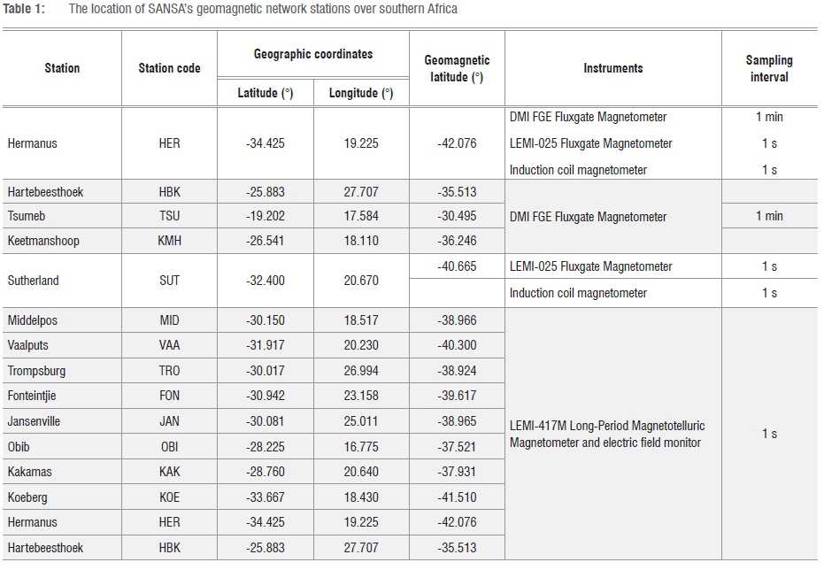
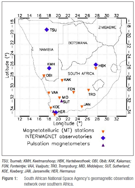
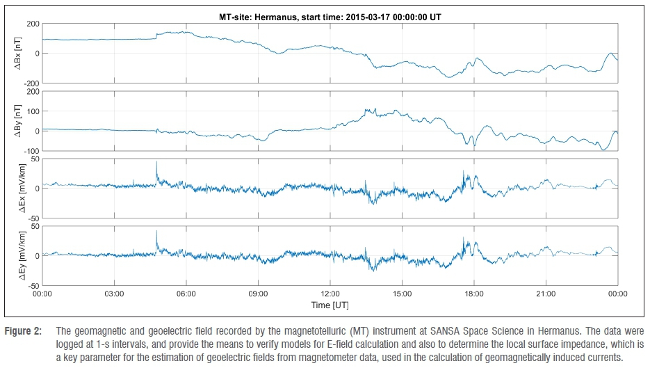
The South African National Space Agency (SANSA) operates four INTERMAGNET (International Real-time Magnetic Observatory Network) observatories in southern Africa: Hermanus (HER) and Hartebeesthoek (HBK) in South Africa, and Tsumeb (TSU) and Keetmanshoop (KMH) in Namibia.9 In addition to these observatories, SANSA operates two induction coil magnetometers for magnetic pulsation data at Hermanus and Sutherland. SANSA operates 10 magnetotelluric stations. The magnetotelluric instrument, a LEMI-417 device (Lviv Center of Institute of Space Research, http://www.isr.lviv.ua/lemi417.htm), of which several are installed in this region, is composed of three magnetic channels to measure the X, Y and Z components of the magnetic field at 1-s intervals, and two electric channels to measure the horizontal components of the electric field at the same location with the same cadence. This network of magnetotelluric stations allows researchers to use measurements of natural geomagnetic and geo-electrical field variations at the earth's surface to model the subsurface electrical conductivity over southern Africa and apply the conductivity to calculate GICs in power grids. The physical locations of these magnetometers and magnetotelluric stations are given in Table 1 and Figure 1.
The largest geomagnetic storm of solar cycle 24 was the severe (G4) storm on Saint Patrick's Day on 17 March 2015.10 The Dst index reached a minimum of -223 nT during this storm.11 In this paper, we look at how SANSA's magnetic network responded to this magnetic storm using local K-indices and show how magnetotelluric stations can be used for the mapping of electric fields and for studying GICs in power networks in southern Africa. The magnetotelluric data from the Hermanus station as recorded on 17 March 2015 are shown in Figure 2.
K-indices
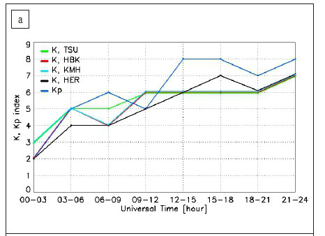
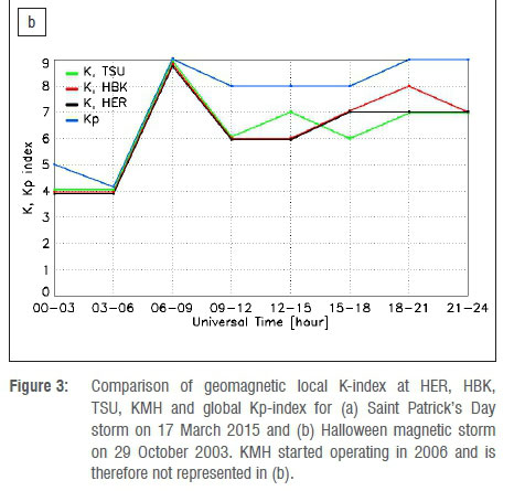
During a geomagnetic storm, temporal geomagnetic variations are the superposition of the regular daily variation, Sq, and the irregular temporal geomagnetic variations. The former is estimated and removed from the signal and the amplitude range indices are calculated based only on the latter. The K-index measures the level of magnetic disturbance and it is derived from the maximum fluctuations of horizontal components relative to the regular 'quiet-time' variation observed during a 3-hour interval. In this study, the linear-phase robust non-linear smoothing (LRNS) method was used in the processing of the magnetic disturbance.12 To compare the local K-indices with a global geomagnetic storm index, we used the Kp-index. For comparison purposes, the Halloween storm on 29 October 2003 was considered. Local K-indices are plotted together with the global Kp-index in Figure 3a and 3b. The trend of the magnetic activity shown by all sets of indices is the same, but the difference in measured magnitude disturbance at the magnetic observatories (Figure 4a and 4b) is significant because it indicates a spatial variation which could have led to non-homogeneity in the E-field over the region during some phases of the storm. This difference can be attributed to latitude dependence of geomagnetic activity, as shown in Figure 4a and 4b for the X and Y components of the geomagnetic field respectively. The variation of the field from one station to another is particularly evident during the main phase of this magnetic storm. Note that the direction of the variation is different for the X and Y components: the magnitude of the disturbed magnetic variation in the X component decreases with latitude, while in the Y component it increases with latitude.
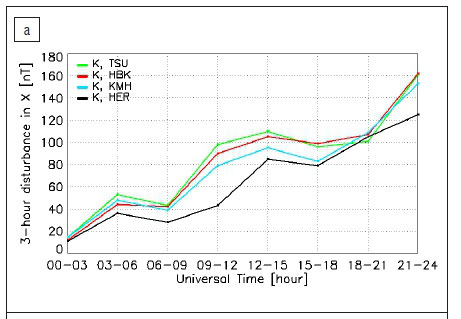
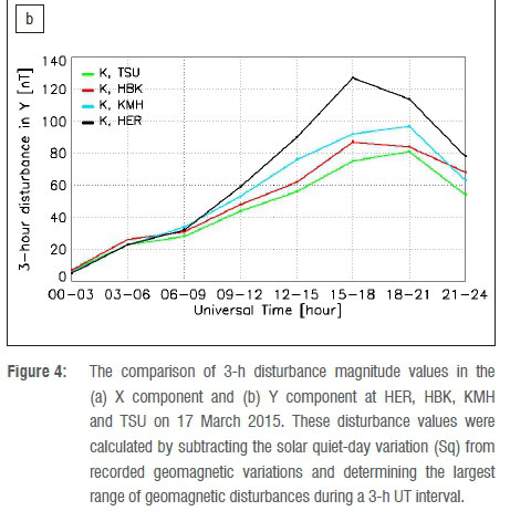
The enhancement in the Y-component disturbance is consistent with disturbances as a result of field-aligned currents, which typically manifest in the dusk to pre-midnight sectors at middle latitudes. The decrease/increase in X/Y disturbance with latitude (Figure 4a and 4b) is indicative of the relative contribution of the ring current related disturbance (enhancing X) diminishing at higher latitudes, and the contribution of the field-aligned current related enhancement (to the Y component) increasing with latitude.13-15
The availability of several observatories in the region is a significant advantage for the characterisation of the latitude dependence of the components of the geomagnetic field. The difference between local K-indices and the Kp-index, and the fact that the differences are not the same for all storms and K-values, makes it necessary to consider local K-indices in the characterisation of storm intensity. In Figure 3a, during the first 12 h of the geomagnetic storm of 17 March 2015, the local K-values are generally lower than or equal to Kp, while during the last 12 h of the storm, the local K-values are consistently lower than Kp. This same trend was also observed for the storm of 29 October 2003 shown in Figure 3b. The difference between Kp- and local K-indices was also observed at other mid-low latitudes INTERMAGNET observatories, namely Fredericksburg (FRD), Kakioka (KAK) and Cheongyang (CYG). The local K-indices are generally smaller than the global Kp-indices specifically for observed planetary geomagnetic disturbances classified as strong, severe or extreme.16 The observation that the variation in the geomagnetic fields at HBK and KMH (on the same latitude and both not coastal) as shown in Figure 3 is about the same (at times during the storm HBK values are slightly higher than those at KMH while at other times they are slightly lower) seems to confirm that stations at the same latitude have similar variations in the geomagnetic field.
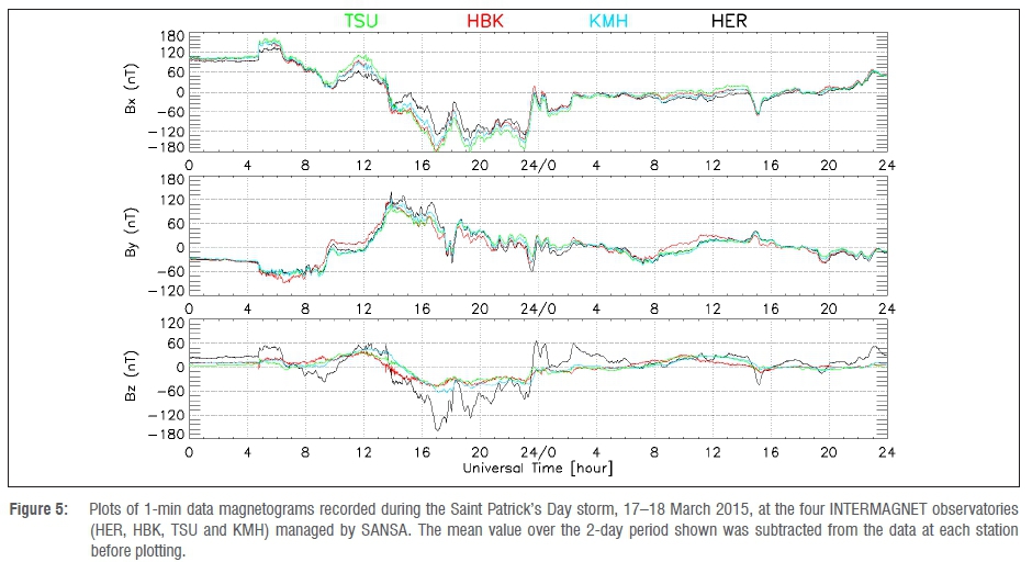
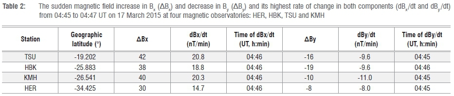
The comparison of magnetograms at the four INTERMAGNET stations - HER, HBK, TSU and KMH - during the storm of 17 March 2015 is shown in Figure 5. The following discussion of the variation of the geomagnetic field includes the storm-related increase and decrease of horizontal (Bx or north directed and By or east directed) and vertical (Bz or downward directed) field components during the storm. The sudden increases in the Bx and Bz components and decrease in the By component are observed at all observatories around 04:45 UT. Table 2 shows the increase in the Bx component from 04:45 to 04:47 UT and the highest rate of change in Bx and By components in this time interval. This marks a sudden storm commencement at 04:45 UT.11 The values in Table 2 show that the highest rate of change in horizontal components during the sudden storm commencement occurred at TSU and the lowest at HER, and HER had the lowest sudden magnetic field increase in Bx and the lowest sudden decrease in the By component. Figure 6a and 6b show the plots of the rate of change in horizontal components, Bx and By, respectively. From Figure 6a it is evident that the maximum rate of change in the Bx component occurred at all four stations during the sudden storm commencement. The largest deviation from the mean over the four stations occurred in the Bz component measured at the Hermanus station, which is closest to the coast. Figure 6b shows that the maximum rate of change in the By component occurred in the Hermanus data and was not during the sudden storm commencement but during the main phase of the storm at about 14:00 and 18:00. The peak values in dBx /dt (20.8 nT/min) were larger than the peak values in dBy /dt (-11 nT/min), which seems to indicate a dominance of the ring current in causing the geomagnetic disturbance. On the other hand, the increase in the variation of the Bz component of the Hermanus observations relative to the variation of the other observatories (Figure 5), and the increase in the maximum dBy/dt from Tsumeb to Hermanus (Figure 6b) is consistent with disturbances resulting from field-aligned currents.13
Geomagnetically induced currents
Geomagnetically induced currents (GIC) have been recorded in the South African power distribution network since 2003. During the geomagnetic storm of 29-31 October 2003, there was a significant impact on the transformers in the network, resulting from thermal damage to power transformers.2 The electric field, which is the primary driver of GIC in the network, has been shown to have a significant spatial variation over southern Africa during a geomagnetic storm, based on the small time differences in the data from different geomagnetic observatories in the region.17 The electric field along every power line is derived from the interpolation of the rate of change of the horizontal components of the geomagnetic field and the surface impedance as derived from local magnetotelluric measurements.18 For the E-field results shown in this paper, the surface impedance derived from the magnetotelluric station in Hermanus was used for calculating the E-field over the whole region of interest. The GIC at any particular grounded transformer is determined by the summation of induced currents in the lines connected to the transformer and the alignment of the power lines connected to the transformer with the electric field. Figure 7a shows the horizontal electric field over southern Africa during the peak of the SSC on 17 March 2015 when the peak electric field magnitude |E| reached 92 mV/km and during the main phase of the storm when |E| reached 53 mV/km. Figure 7b shows the spatial distribution of the horizontal component of the E-field during a time when there was a maximum spatial variation in the direction of the E-field. Figure 7a shows that the variation in magnitude and direction of the E-field is minimal during the period when the E-field was high. On the other hand, Figure 7b shows that both the magnitude and the direction of the E-field exhibit a significant spatial variation during other times of the storm. The spatial variation shown in Figure 6b does not provide strong evidence of either a latitudinal or coastal effect. The coastal effect - namely an increase in the component of the E-field perpendicular to the coast on the landside at locations close to the land-ocean boundary - is a result of the increase in the conductivity of the earth moving from land to sea. This increase is physically a result from charge accumulation at the land-ocean boundary.19 In Figure 7b there is evidence of both an increase of the E-field towards the ocean along the line from KMH to HER (Figure 7b, left panel) and at another time a decrease in the E-field towards the ocean along the line from KMH to HER (Figure 7b, right panel). This observation is attributed to the fact that a uniform surface impedance was used for the calculation of the E-field at all grid points, including those over the ocean, and that the phase differences in the E-field which give rise to spatial turbulence supersede the latitudinal and coastal effects.
Discussions
At coastal observatories, like HER, geomagnetic variations are more intense than elsewhere along the same latitude because of the close proximity of salty seawater. This coastal effect is the strongest in the vertical Z-component of the geomagnetic field20 while the horizontal components like X and Y behave differently. The coastal effect is clearly illustrated during the Saint Patrick's Day storm in Figure 5 where the Z component at HER showed significant differences, particularly during the main phase from 14:00 on 17 March 2015. We also noticed that the induction effect of the ocean at HER is not constant and that it varied with time as the storm developed, with the largest deviation of approximately 65 nT to be observed around 17:00 UT. Hartebeesthoek, located 1250 km to the northeast of Hermanus, does not show a measurable coastal contribution, while Tsumeb, which is about 1500 km north of Hermanus, is influenced by a small induction disturbance.
There is a further enhancement in the electric field close to the coast because of the abrupt change in the surface impedance near the coast. Modelling done by Gilbert21 has shown that the enhancement to the component of the electric field directed perpendicular to the coast behaves as the inverse of the square root of the distance from the shoreline and this effect extends to a distance on the order of a skin depth inland.
The peak magnitude of the electric field |E| over southern Africa was estimated at 92 mV/km and occurred at 04:46 UT on 17 March 2015 during the SSC phase of the storm. Although no damage to the South African power network has so far been attributed to the impact of the Saint Patrick's Day storm, the peak magnitude of the electric field |E| over southern Africa was in the same order of magnitude as the peak E-field during other storms during which damage was caused in the power network. This peak was about 63% of the peak of 147 mV/km estimated to have occurred at the peak of the 2003 Halloween geomagnetic storm which occurred during the main phase of the storm at 06:40 UT on 29 October 2003 which had a significant impact on the South African power network.20 The difference in the impact may be attributed not only to the peak value of the E-field, but also to the duration of large values of |E| being longer during the 2003 storm, which is more likely to have caused thermal damage. Note that the E-field was predominantly westward during the period shown in Figure 7a, but turned eastward during the main phase of the storm. During the main phase of the storm of 17 March 2015, the highest value of |E| was 53 mV/km, which occurred at 13:55 UT. Such variations in the magnitude and direction of the magnetic field can only be determined because data are available from a regular distribution of magnetic observatories as in southern Africa, as the spatial variation in both magnitude and direction of the E-field at any particular time during the storm could not be inferred properly from the observations at only a single observatory in the region. The components of the E-field that are parallel and perpendicular to the coast are affected in opposite ways. The parallel component decreases with proximity to the coast while the perpendicular component increases with proximity to the coast.21 During the peak of the storm, the E-field has a fairly homogeneous spatial distribution over the region (Figure 7a) but during other times the E-field is turbulent (Figure 7b) and exhibits both an increase in magnitude with proximity to the coast (KMH to HER, Figure 7b, left panel), and a decrease in magnitude (KMH to HER, Figure 7b, right panel), which seems to supersede the latitudinal and coastal effects. The scale length of the variations in the E-field during the most turbulent parts of the storm, as shown in Figure 7b, is in the order of the spacing between the observatories.
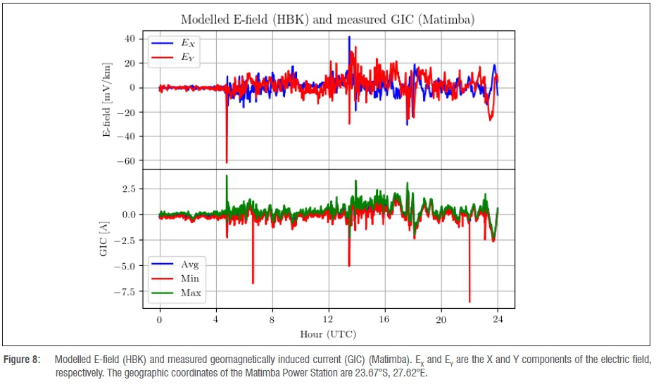
Figure 8 shows GIC recorded at a generating power station in northern South Africa for 17 and 18 March 2015, with the electric field calculated at HBK according to the Grassridge ground conductivity profile. As far as we are aware, the GIC amplitude, with maximum of about 8 A, was too small to cause significant immediate damage to infrastructure. Records of degradation leading to failures of several transformers after the Halloween geomagnetic storm in 2003, and attributed to GICs, have indicated much smaller currents could initiate damage.2 Transformer failures attributed to even lower GICs (less than 8 A in the neutral) were reported from the UK22 with peaks in modelled Ex and Ey, corresponding to storm commencement and main phase, coinciding with peaks in recorded GIC. The GIC currents were measured in the neutral to ground connection of a Y-connected transformer. The sampling rate of the GIC measurements is not known. The only parameters recorded by the power utility are the maximum, minimum and mean values over every 5-min interval. In Figure 8, the minima that have been measured at about 06:30 and 22:00 UTC which are not correlated to peaks in the E-field, could indeed be spikes that are unrelated to the real disturbance. The correlation coefficients of the average GIC with the 5-min averages of Ex and Ey components are -0.6595 and 0.41266, respectively.
Conclusion
The geomagnetic observation network of SANSA in southern Africa plays a crucial role in the proper identification and characterisation of the spatial distribution of disturbance effects resulting from geomagnetic storms. We have shown data for several locations throughout the storm, which reveal the spatial distribution over the region of the storm-related geomagnetic variations. The inhomogeneity at significantly lower values of the calculated E-field during the main phase of the storm resulting from the variation in the geomagnetic field over the region has been demonstrated. The data show that there are differences between global and local indices, which vary with the phases of the storm. The increase in the dB/dt as a result of the coastal effect has been demonstrated. The contributions made by ocean induction on observatory data located near the coast, particularly during magnetic disturbances, can be further investigated using high-precision magnetic satellite data like Ørsted, CHAMP and SWARM. The impacts of the coastal effects on the electric field during geomagnetic disturbances can be further investigated by using measured GIC data from coastal power stations such as the Koeberg Nuclear Power Station on the coast near Cape Town.
Acknowledgements
Eskom is acknowledged for providing the GIC data measured at the Matimba Power Station. The results presented in this paper rely on the data collected at Hermanus, Hartebeesthoek, Tsumeb and Keetmanshoop Observatories. We thank SANSA for supporting their operation and INTERMAGNET (www.intermagnet.org) for promoting high standards of magnetic observatory practice.
Authors' contributions
E.N.: Writing the first draft of the manuscript, analysing data, participating in the manuscript revision and putting together the contributions from other authors. P.B.K.: Revision of the manuscript for its improvement. P.J.C.: Supporting the writing of the first draft, analysing data and participating in the manuscript revision for its improvement. S.L.: Analysing data and revision of the manuscript for its improvement.
References
1.Turnbull KL, Wild JA, Honary F, Thomson AWP, McKay AJ. Characteristics of variations in the ground magnetic field during substorms at mid latitudes. Ann Geophys. 2009;27:3421-3428. https://doi.org/10.5194/angeo-27-3421-2009 [ Links ]
2.Gaunt CT, Coetzee G. Transformer failures in regions incorrectly considered to have low GIC-risk. IEEE PowerTech, Lausanne. 2007:807-812. https://doi.org/10.1109/PCT.2007.4538419 [ Links ]
3.Kamide Y, Balan N. The importance of ground magnetic data in specifying the state of magnetosphere-ionosphere coupling: A personal view. Geosci Lett. 2016;3, Art. #10, 8 pages. https://doi.org/10.1186/s40562-016-0042-7 [ Links ]
4.Thomsen MF. Why Kp is such a good measure of magnetospheric convection. Space Weather. 2004;2(11), S11004, 10 pages. https://doi.org/10.1029/2004SW000089 [ Links ]
5.Bartels J, Heck NH, Johnston HF. The three-hour-range index measuring geomagnetic activity. J Geophys Res. 1939;44:411-418. https://doi.org/10.1029/TE044i004p00411 [ Links ]
6.Bartels J. The standardized index, Ks, and the planetary index, Kp. IATME Bull. 1949;13b:97. [ Links ]
7.Sugiura M. Hourly values of equatorial Dst for the IGY. In: Annals of the International Geophysical Year. Vol. 35. New York: Elsevier; 1964. p. 945-948. [ Links ]
8.Echer E, Gonzalez WD, Alves MV. On the geomagnetic effects of solar wind interplanetary magnetic structures. Space Weather. 2006;4(6), S06001, 11 pages. https://doi.org/10.1029/2005SW000200 [ Links ]
9.Kotzé PB, Cilliers PJ, Sutcliffe PR. The role of SANSA's geomagnetic observation network in space weather: A review. Space Weather. 2015;13(10):656-664. https://doi.org/10.1002/2015SW001279 [ Links ]
10.Kamide Y, Kusano K. No major solar flares but the largest geomagnetic storm in the present solar cycle. Space Weather. 2015;13(6):365-367. https://doi.org/10.1002/2015SW001213 [ Links ]
11.Wu C, Liou K, Lepping RP, Hutting L, Plunkett S, Howard RA, et al. The first super geomagnetic storm of solar cycle 24: 'The St. Patrick's Day event (17 March 2015)'. Earth Planets Space. 2016;68, Art. #151, 12 pages. https://doi.org/10.1186/s40623-016-0525-y [ Links ]
12.Hattingh M, Loubser L, Nagtegaal D. Computer K-index estimation by a new linear-phase, robust, nonlinear smoothing method. Geophys J Int. 1989;99:533-547. https://doi.org/10.1111/j.1365-246X.1989.tb02038.x [ Links ]
13.Sun W, Ahn B, Akasofu S. A comparison of the observed mid-latitude magnetic disturbance fields with those reproduced from the high-latitude modeling current system. J Geophys Res Space Phys. 1984;89(A12):10881-10889. https://doi.org/10.1029/JA089iA12p10881 [ Links ]
14.Nakano S, Iyemori T. Storm-time field-aligned currents on the nightside inferred from ground-based magnetic data at mid-latitudes: Relationships with the interplanetary magnetic field and substorms. J Geophys Res Space Phys. 2005;110(A7), A07216, 13 pages. https://doi.org/10.1029/2004JA010737 [ Links ]
15.Vennerstrom S, Christiansen F, Olsen N, Moretto T. On the cause of IMF By related mid- and low latitude magnetic disturbances. Geophys Res Lett. 2007;34(16), L16101, 5 pages. https://doi.org/10.1029/2007GL030175 [ Links ]
16.Yi W, Kim J. Comparison of planetary and local geomagnetic disturbance indices: Operational implications. J Atmos Solar-Terrestrial Phys. 2018;178:1-6. https://doi.org/10.1016/j.jastp.2018.04.016 [ Links ]
17.Bernhardi EH, Tjimbandi TA, Cilliers PJ, Gaunt CT. Improved calculation of geomagnetically induced currents in power networks in low-latitude regions. In: Proceedings of the 16th Power Systems Computation Conference; 2008 July 14-18; Glasgow, Scotland. New York: Curran Associates Inc.; 2010. p. 1391-1395. [ Links ]
18.Bernhardi EH, Cilliers PJ, Gaunt CT. Improvement in the modelling of geomagnetically induced currents (GICs) in Southern Africa (SA). S Afr J Sci. 2008;104:265-272. [ Links ]
19.Pirjola R. Practical model applicable to investigating the coast effect on the geoelectric field in connection with studies of geomagnetically induced currents. Adv Appl Phys. 2013;1(1):9-28. https://doi.org/10.12988/aap.2013.13002 [ Links ]
20.Olsen N, Kuvshinov A. Modelling the coastal effect of geomagnetic storms. Earth Planets Space. 2004;54:525-530. https://doi.org/10.1186/BF03352512 [ Links ]
21.Gilbert JL. Modeling the effect of the ocean-land interface on induced electric fields during geomagnetic storms. Space Weather. 2005;3, S04A03, 9 pages. https://doi.org/10.1029/2004SW000120 [ Links ]
22.Erinmez IA, Kappenman JG, Radasky WA. Management of the geomagnetically induced current risks on the National Grid Company's electric power transmission system. J Atmos Solar-Terrestrial Phys. 2002;64:743-756. https://doi.org/10.1016/S1364-6826(02)00036-6 [ Links ]
 Correspondence:
Emmanuel Nahayo
enahayo@sansa.org.za
Received: 05 June 2018
Revised: 19 July 2018
Accepted: 19 Oct. 2018
Published: 30 Jan. 2019
Supplementary Material
The open data set is available here: [Open data set]

