


Services on Demand
Article
 English (pdf)
 Article in xml format
 Article references
Indicators

Related links
-
 Cited by Google
 -
 Similars in Google
Share

 Permalink
South African Journal of Science
On-line version ISSN 1996-7489
Print version ISSN 0038-2353
S. Afr. j. sci. vol.114 n.9-10 Pretoria Sep./Oct. 2018
http://dx.doi.org/10.17159/sajs.2018/4841
RESEARCH ARTICLE
Mapping chlorophyll-a concentrations in a cyanobacteria- and algae-impacted Vaal Dam using Landsat 8 OLI data
Oupa E. MalahlelaI; Thando OliphantII; Lesiba T. TsoelengI; Paidamwoyo MhangaraI
IResearch and Applications Development, Earth Observation Directorate, South African National Space Agency, Pretoria, South Africa
IIData Products and Services, Earth Observation Directorate, South African National Space Agency, Pretoria, South Africa
ABSTRACT
Mapping chlorophyll-a (chl-a) is crucial for water quality management in turbid and productive case II water bodies, which are largely influenced by suspended sediment and phytoplankton. Recent developments in remote sensing technology offer new avenues for water quality assessment and chl-a detection for inland water bodies. In this study, the red to near-infrared (NIR-red) bands were tested for the Vaal Dam in South Africa to classify chl-a concentrations using Landsat 8 Operational Land Imager (OLI) data for 2014-2016 by means of stepwise logistic regression (SLR). The moderate-resolution imaging spectroradiometer (MODIS) data were also used for validating chl-a concentration classes. The chl-a concentrations were classified into low and high concentrations. The SLR applied on 2014 images yielded an overall accuracy of 80% and kappa coefficient (κ) of 0.74 on April 2014 data, while an overall accuracy of 65% and κ=0.30 were obtained for the May 2015 Landsat data. There was a significant (p<0.05) negative correlation between chl-a classes and red band in all analyses, while the NIR band showed a positive correlation (0.0001; p<0.89) for April 2014 data set. The 2015 image classification yielded an overall accuracy of 83% and κ=0.43. The difference vegetation index showed a significant (p<0.003) positive correlation with chl-a concentrations for May 2015 and July 2016, with chl-a ranges of between 2.5 µg/L and 1219 µg/L. These correlations show that a class increase in chl-a (from low to high) is in response to an increase in greenness within the Vaal Dam. We have demonstrated the applicability of Landsat 8 OLI data for inland water quality assessment.
Significance:
• The magnitude of the algae problem in the Vaal Dam is highlighted.
• Landsat 8 OLI satellite data have potential in mapping chl-a in inland water bodies.
• Both the red and the near infrared wavelengths were significant in mapping chl-a concentrations in the Vaal Dam.
• Satellite earth observation can be instrumental for water quality monitoring and decision-making.
Keywords: chlorophyll-a; Landsat 8; Vaal Dam; water quality
Introduction
Freshwater resources are central for human sustenance and are a catalyst for economic development. However, freshwater resources globally are increasingly being polluted by industrial effluent, phosphorous and residual nitrates1 attributed to rapid industrialisation2, and the intensive use of fertilisers and pesticides in agriculture3. This situation is becoming more precarious in industrialised and agrarian economies with scarce surface freshwater resources. For many years, the subject of water quality has attracted the attention of policymakers and scientists across the African continent.4,5 South Africa, in particular, is currently confronted with several water quality issues. Eutrophication is at the centre of water quality challenges currently confronting water authorities in South Africa, and is a matter of public and scientific concern.6 Satellite-based remote sensing is increasingly playing a fundamental role in providing valuable spatial and temporal measurements of the concentration of chlorophyll-a (chl-a) in water bodies dominated by cyanobacteria and algal blooms globally. Many scientific studies have highlighted the advantages of using satellite imagery in monitoring the status of eutrophication in case II water bodies regularly.7,8 Thus, the estimation of chl-a concentration in inland water bodies is important for effective monitoring of water quality for management purposes.
However, determination of light-absorbing chl-a in case II water bodies (those water bodies whose optical properties are determined by phytoplankton and related constituents9) is more challenging considering the optical properties of the water bodies. This challenge is primarily because of the presence of other biophysical constituents such as dissolved organic matter and suspended solids with varying abundance, concentrations and reflectance.10,11 This variation leads to a situation in which the chl-a concentrations do not necessarily present a readily measureable, homogenous surface cover across the water body. Instead, complex optical properties are realised, thereby increasing challenges related to chl-a detection.11 Fortunately, remote sensing technology has opened avenues for successful detection of chl-a concentrations in inland water bodies, through prevalence of algae12 and aquatic invasive vegetation13-15.
One of the most commonly used remote sensing approaches for deriving chl-a is hyperspectral sensing, which has proved effective for estimating chl-a in case II waters.11,16,17 However, the use of hyperspectral data and models is limited by its cost and high data dimensionality. In order to address this challenge, a number of optical multispectral sensors, such as the moderate-resolution imaging spectroradiometer (MODIS) and medium-resolution imaging spectrometer (MERIS) were used for estimating chl-a in inland waters.11,18,19 The application of MODIS and MERIS to estimate chl-a concentrations is possible mainly because of the relationship between chl-a concentrations and spectral reflectance in red and near-infrared (NIR) regions.20,21 However, the coarse spatial resolution of MODIS and satellite discontinuity of MERIS have made it challenging to map chl-a to resolve small water bodies, particularly when mapping relies on the complementary nature of MODIS data by MERIS data sets. Additionally, the low signal-to-noise ratio of these sensors (8-bit) may not be adequate to characterise inland water quality.
The advancement in remote sensing technology has resulted in the launch of Landsat 5 Thematic Mapper (TM) and 7 Enhanced Thematic Mapper (ETM+) space-borne sensors with a spatial resolution of 30 m. These sensors comprise spectral regions similar to those of the MODIS sensor, in the visible to NIR region. Both Landsat 5 and 7 have demonstrated superior capability to both MERIS and MODIS in medium-size and small inland water as a result of their spatial resolution.22 They are known to be characterised by limited signal-to-noise ratio, four bands in the visible-NIR, and an 8-bit quantiser.23 However, the instrumentation problems associated with Landsat 7 image acquisition limit the applicability of this sensor in detecting moving algal concentrations. For example, the Scan Line Corrector (SLC; an electromechanical device that compensates for the forward motion of Landsat 7) failed on 31 May 2003, resulting in up to 22% of the pixels missing in the collected image scenes.24 The recently launched Landsat 8 Operational Land Imager (OLI) with improved signal-to-noise ratio and 12-bit quantisation exhibited the potential to map chl-a by using empirical band ratio regression models.25 This potential is because of its stripe-free images, as opposed to the striped images acquired by Landsat 7 ETM+ over the local study area. Based on the assumptions made by Gitelson et al.26 and Dall'Olmo and Gitelson27 regarding the sensitivity of red and NIR bands in estimating chl-a, the question arose as to whether we can effectively use Landsat OLI data to map such chl-a concentrations in water bodies whose properties are significantly affected by mineral particles (i.e. case II water bodies).
Various statistical models have been used to map chl-a in both case I and II waters. Case I water consists of a high concentration of phytoplankton compared to other particles, whereas case II waters consist of high turbid water with an abundant occurrence of dissolved organic matter and suspended solids. Amongst these different algorithms is the linear inversion matrix28, neural network methods13,29 and regression models30. Perhaps one of the most commonly used methods is the linear regression model, which relates water/chl-a concentrations to spectral measurements as observed by satellites.31 There are limited studies that have used the logistic regression model, which is a type of generalised linear model, for estimation of chl-a, particularly when such estimations are done to categorise chl-a into discreet classes. Therefore, we aimed to estimate chl-a concentrations of cyanobacteria and algae in the Vaal Dam in South Africa using the Landsat 8 OLI data set. The objective of the study was to test whether single and two-band normalised indices, derived from sensitive bands, could aid in estimating chl-a concentrations in the Vaal Dam. The Vaal Dam is one of the largest and economically most important dams in South Africa, with its significance highly recognised, particularly during the dry season.32 To the best of our knowledge, there has never been a study in South Africa in which Landsat OLI data were used in modelling chl-a concentrations in large, semi-arid water bodies such as the Vaal Dam. Spatial data concerning the concentrations of chl-a in economically important dams of South Africa remain limited.
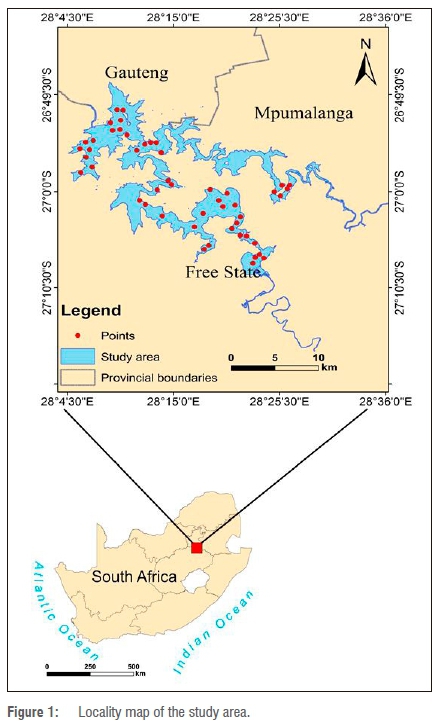
The Vaal Dam is a trans-provincial water body that forms a boundary between the Gauteng and Mpumalanga Provinces, Gauteng and Free State Provinces, and Free State and Mpumalanga Provinces of South Africa. It is located at 26°56'49''S and 28°14'30''E (Figure 1). The dam was constructed in 1938 with a wall height of 54.2 m, which was elevated to 63.5 m in 1985 because of increased water capacity of 2188 million m3/year.33 The Vaal Dam has a surface area of approximately 321 km2 and an average depth of 22.5 m; and the Dam supplies large volumes of water to the people of South Africa.34 The water is mostly turbid, with the Dam characterised by silty bottom strata responsible for constant turbidity at varying degrees. Apart from the turbid nature of the Dam, algal blooms that affect the biophysical and chemical quality of the water are a growing concern35; these blooms are a common phenomenon along the Vaal River System. Because of its economic importance, there is a need to monitor algal blooms and to control cyanobacteria - which are the primary indicators of eutrophication levels in case II waters - within this reservoir. Cyanobacterial blooms have been a major environmental concern for many years, with well-known cattle deaths in the 1940s associated with cyanobacteria.36 Although there is sufficient public awareness of the impacts of cyanobacteria in South Africa, information on the spatial distribution of chl-a over time within the Vaal Dam is lacking, and is crucial for reservoir management.
Methods
Data and pre-processing
Landsat 8 OLI data were explored as a source to estimate chl-a concentrations of cyanobacteria and algae within the Vaal Dam. Table 1 shows the details of images acquired for the study. One of the images was acquired on 22 April 2014 - the day that corresponded to one of the highest peaks of algal blooms in water bodies in the Vaal Dam.37 Landsat 8 data comprise a total of 11 spectral bands in the visible to thermal infrared region (0.43-12.51 µm). In the visible shortwave infrared spectrum, Landsat 8 has a band range from coastal band (0.44 µm) to shortwave infrared (2.29 µm) and a ground sampling distance of 30 m. Each of the spectral bands in the visible shortwave infrared range was converted from a digital number to top-of-atmosphere reflectance value (0-1) by means of Equation 1:
ρλ' = ρM Qcal + ρA Equation 1

where ρλ is top-of-atmosphere planetary reflectance, without correction for solar angle; ρM is a band-specific multiplicative rescaling factor, ρA is the band-specific additive rescaling factor, and Qcal is the quantised and calibrated standard pixel values in digital numbers.38 Based on our objective, a total of seven (7) spectral bands were merged to form multispectral images with 16-bit radiometric resolution. These spectral bands were coastal (0.44 µm), blue (0.48 µm), green (0.56 µm), red (0.66 µm), near-infrared (0.87 µm), shortwave infrared1 (1.61 µm) and shortwave infrared2 (2.20 µm). The atmospheric correction processing was done on each satellite image using Quick Atmospheric Correction (QUAC) module in ENVI®.39 The resultant QUAC images had values from 0 to 10 000, and were rescaled to have values of between 0 and 1 using Equation 2:
Imgn = Imgi x 0.0001 - 0.1 Equation 2
where Imgn is the new reflectance image (0-1 value) and Imgi is the QUAC image with values scaled to 10 000. This step was necessary to allow for comparison of image values after the effect of atmosphere was removed from the images. The QUAC algorithm was chosen because of its accuracy in chl-a estimation for turbid waters and because it comes as a standard extension in the ENVI software.38,39
In order to derive the geographical extent of the Vaal Dam from satellite images, a simple water index algorithm was applied on individual images. The index is based on the low within-class variation of water pixels in blue (0.48 µm) and shortwave infrared (1.61 µm) bands of Landsat 8 OLI. It classifies water pixels as 1 and non-water pixels as 0 and has shown to be effective in many parts of the world.38 This processing was followed by subsetting an atmospherically corrected 7-band Landsat OLI imagery of the delineated study area. Ultimately, the pre-processing included pan-sharpening of the individual image with a 15-m panchromatic band in order to improve the ground sampling distance of the 30-m images using the nearest-neighbour resampling method.
Selecting regions of interest
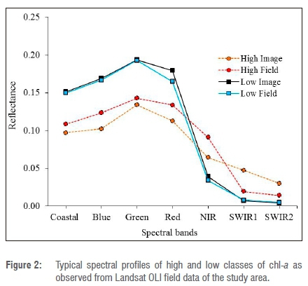
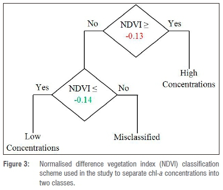
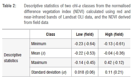
The visual interpretation of various chl-a densities was done on pan-sharpened Landsat 8 imagery (15 m ground sampling distance) in order to extract regions of interest (ROIs). The ROIs were chosen with the aid of the spectral reflectance curve shown in Figure 2 and the two-class algorithm based on the normalised difference vegetation index (NDVI) shown in Figure 3. The spectral profiles were pre-assessed using average spectra of extracted pixels from the 2016 image classes (low=17 and high=6) corresponding to field data collected during this period. Figure 2 shows that average spectra of the low and high chl-a classes for both visual (image data set) and quantitative (field data set) selection are not very different from each other. Additionally, Table 2 gives a summary of the statistics of low and high chl-a classes derived from Landsat data and field data collected on the Vaal Dam. A total of 49 (n=49) ROIs was extracted from each image, corresponding to images acquired in 2014 to 2016. The ROIs were chosen to fall within low or high chl-a concentration classes.
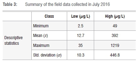
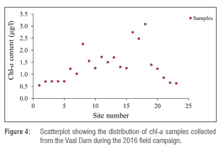
Field data were collected on 16 July 2016 from the Vaal Dam. Sampling was done in terms of the exact longitudes and latitudes of the sampling points and in-situ classification of chl-a concentration; actual algae samples were taken for laboratory analysis. The data were collected corresponding to the time of the Landsat 8 OLI overpass (at approximately 10:00). A total of 23 samples was collected and all samples were analysed for chl-a concentration. Table 3 gives the details of the field data collected. This data set was used for validating the model used for predicting chl-a and was later used for producing the maps. Figure 4 shows the scatterplot of the points collected in the field. Because the minimum chl-a value (2.5 µg/L) was far less than the maximum chl-a value (1219 µg/L), we applied the log transformation to this skewed data using Logx+1 in order to force the data to conform to normality.
Data analysis
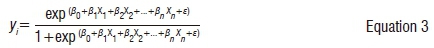
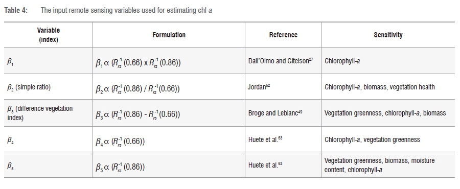
Data analysis was performed on three Landsat images in R,40 QGIS version 2.12 and ENVI version 4.7. Various vegetation indices that are sensitive to chl-a were derived. These indices, in addition to chl-a sensitive bands, were selected on the basis of their relationship with chl-a in case II water bodies.26 These indices were two-band indices in the red-NIR region of Landsat OLI. Table 4 shows the vegetation indices used in this study. From each image, 60% of the ROIs (n=29) was used for training the model, while 40% (n=20) was reserved as an independent validation data set. Similar ROIs were used for calibrating the model for the 2016 image, with the field data set serving as validation. In order to estimate classes of chl-a using remote sensing data, a multiple step-wise logistic regression (SLR) was employed. The SLR is given in the form of:
where y is the resultant chl-a concentration of an i-th class, a is the y-intercept, bn is the regression estimate of variable xn, and ɛ is an error associated with prediction which was not pre-determined but it is associated with the logistic regression model. In addition, the D2 (which is an analogy of R2) was used to compare the strength of the model fit. The D2 is given by:

Because we were using images acquired on different dates, it was necessary to assess possible differences and similarities between ROIs collected from the 2016 image (date of field data acquisition) and those collected from 2014 and 2015 images. For this reason, we adopted the spectral discrimination index (SDI) for the 2014/2016 image pair and the 2015/2016 image pair41,42 acquired for the same season (autumn). The SDI is computed from Equation 5 as:
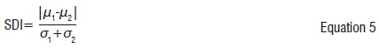
where µ1 and µ2 are the mean values of chl-a pixels in time period 1 and 2, respectively; and σ1 and σ2 are the standard deviations of the chl-a pixels between time 1 and 2, respectively. A higher SDI indicates that these two images are significantly different while a lower value indicates that there is a form of similarity in conditions at times 1 and 2. A rule of thumb is that an SDI>1 shows a satisfactory dissimilarity between two mean values. The preliminary SDI on extracted ROIs showed less varying chl-a spectra on Landsat 8 OLI images acquired in 2014-2016 (µ2014=0.090, s.d.=0.053; µ2015=0.103, s.d.=0.083; µ2016=0.084, s.d.=0.037). The SDI value between 2014 and 2016 images was 0.07, while a value of 0.16 was obtained on images acquired in 2015 and 2016. This information suggested that the spectral analysis could further be done for all three image dates as the conditions prevailing during field data collection did not significantly differ (SDI<0.2).
Accuracy assessment
In order to validate the reliability of the results and model used in estimating two main classes of chl-a concentrations, statistical comparison was done between the predicted chl-a and visually quantified chl-a. For a more robust validation of the model, the field data collected on 16 July 2016 were used as an independent validation data set (n=23), which was not significantly different from the data set used for 2014 and 2015 validation (n=20). The NDVI derived from MODIS was used against the predicted classes. The MODIS data were used for evaluating any similarities between MODIS NDVI and Landsat 8 NDVI used to classify chl-a preliminarily into high and low classes. The NDVI is the quantitative indicator of vegetation greenness and its relative density as observed using space-borne satellites. The NDVI values have a range from -1.0 to +1.0, with positive values (close to +1.0) indicating healthy green pigment. Geographical features such as water, areas of barren rock, sand, and bare soil are usually characterised by values below zero (close to -1.0).
The MODIS NDVI product has shown correlation with various chl-a classes and the ground data in Heihe River Basin, with an R2 of up to 0.98.43 On the other hand, Gitelson et al.44 have shown that MODIS-retrieved NDVI vs fAPARgreen showed a very close relationship with the fAPARgreen vs in-situ NDVI, while MODIS NDVI showed positive correlation with chlorophyll content45. This makes the MODIS NDVI product a good reference data set for chl-a studies. The reference data set was obtained from points generated on MODIS NDVI with 250-m pixel resolution, and the ROIs from Landsat 8. The MODIS NDVI products were produced for the dates that correspond with the Landsat 8 image acquisitions for 2014 and 2015, as the 2016 data set could only be validated using the field data set. Because MODIS NDVI values are scaled from -1999 to 7500, we converted them to standard NDVI values of between -1.0 and 1.0 using Equation 6:
NDVIn = NDVI x 0.0001 Equation 6
where NDVIn is the standard NDVI, and NDVI is the MODIS NDVI product. Classification accuracy was computed from the overall accuracy, which is the total number of correctly classified cases to the total number of cases. In addition, the accuracy was further assessed by calculating the kappa coefficients (κ) between classes of low chl-a concentrations (0) and high concentrations (1) using the field chl-a data set. The κ is given by:

where ρobs is the observed proportion of agreement and ρchn is the proportion expected by chance.
Results and discussion
The results of the SLR are shown in Table 5. The SLR model used to estimate classes of algae based on chl-a concentration was more sensitive for the April 2014 analysis than for both May 2015 and 2016 data sets. For the April 2014 Landsat data, the SLR model yielded a higher D2 than for the May 2015 data (D2=76.8% and 35.01%, respectively). The April period in South Africa corresponds to the period when the algae and cyanobacteria in the Vaal Dam reach their maximum photosynthetic activities.37 Classification of the 2016 image yielded the second highest D2 of 64.37%. The equations used to derive chl-a distribution maps (classes) for both April 2014 and May 2015 are given by:
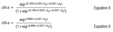
Equations 8 and 9 were applied to the 2014 and 2015 images, respectively. The model which comprises variables β4 (red band at 0.66 µm) and β5 (NIR band at 0.86 µm) as predictors was used for estimating chl-a concentration in the Vaal Dam. The red band (β4) was significantly and negatively correlated with the density of chl-a in the dam (-0.002; p<0.001) for the April 2014 Landsat 8 data. This relationship is as a result of the photochemical activity of photosystem II which is characterised by a reduction in the shorter wavelength red band because of increased chl-a concentration.46 Additionally, although not significantly, the NIR band (β5) was positively correlated with the density of chl-a (0.0001; p<0.89). The positive correlation between the chl-a and the NIR also supports the negative correlation between the red band and chl-a density. The increase in algae biomass results in an increase in the opposing trends between the NIR and red band correlations (Figure 3). The NIR region, which is outside of the PAR region, is mainly used by the algae for photomorphogenesis, which is light regulating changes in development, morphology, biochemistry, cell structure and function in response to light.47,48
For the 2016 winter image, the estimation of chl-a was derived following Equation 10. The pattern of this model used for predicting chl-a concentration showed similarity to the one used in 2015.
On the other hand, the difference vegetation index represented as variable β3 was the only significant (0.0027; ρ<0.018) remote sensing variable for predicting chl-a in the Vaal Dam for the images acquired in both May 2015 and July 2016. The positive correlation between chl-a classes and difference vegetation index suggests that the higher the concentration of the healthy green algae, the greater the absorption of the red band (PAR), as the difference vegetation index is calculated from the difference between the red and NIR bands.49 It is generally known that remote sensing indices are better designed for mapping changes in chl-a than are individual spectral bands because of their ability to compensate for errors resulting from solar or viewing geometry.
Initial desktop validation data showed that the SLR model applied on Landsat OLI April 2014 data yielded an 80% overall accuracy while a 65% overall accuracy was obtained from Landsat OLI data for May 2015. There was substantial agreement (κ=0.74) between the validation data set and the predicted chl-a concentrations for the image acquired on 22 April 2014, while a fair agreement (κ=0.30) was observed for the 22 May 2015 image. These levels of agreement were predominantly affected by the sample size of the validation data set. However, the field data set resulted in a classification accuracy of 83% with fair agreement between the observed and the measured concentrations (κ=0.43).
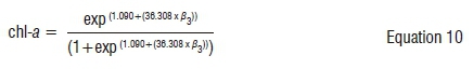
Thematic maps
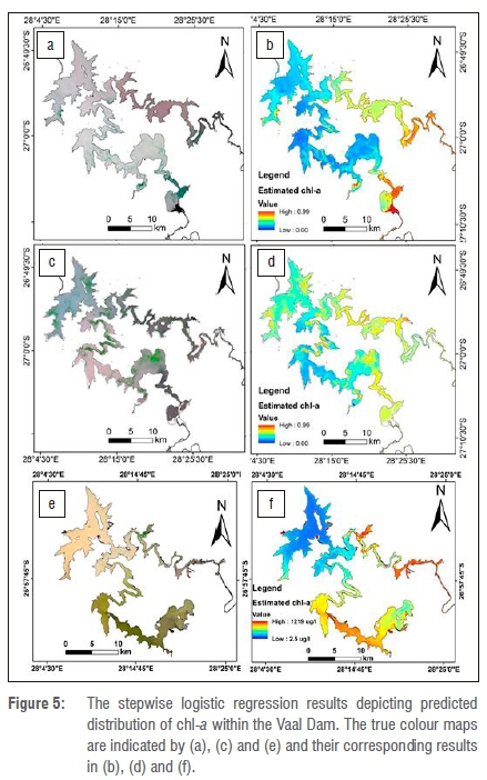
Figure 5 shows the results of the spatial characteristics of predicted chl-a for the April 2014 and May 2015 study periods. The chl-a concentration ranged from 0 (indicating low class) to 0.99 (indicating high class) in the lentic freshwater body corresponding to a minimum of 2.5 µg/L and a maximum of 1219 µg/L. On the other hand, there is correlation (R2=0.61) between the log-transformed chl-a measurements and the estimated chl-a as shown in Figure 6. The resultant maps indicate that higher class concentrations were predominantly found at or near the shores of the dam. These areas are usually shallower with higher temperatures than the deep waters, resulting in lateral diurnal thermal variations.50 In addition, the various concentrations of algal blooms are also attributed to the global changes in climate and anthropogenic activities.51 Whereas climate change affects algal formation at a global scale, the local anthropogenic activities - such as nutrient load into the Vaal Dam - are more important in controlling algal densities. This is particularly important considering the various forms of human activities occurring at different parts of the Vaal River Basin. The higher concentrations were usually found where the Dam has a meandering shape, especially in the northern part of the Dam, although some higher chl-a concentrations occurred within the Dam. The northern part is where the Vaal River flows into the Vaal Dam, contributing a greater proportion of nutrient load.52
From the Landsat data acquired for April 2014, high concentrations of chl-a were estimated to be in the southeasterly part of the Dam - a flood plain composed mainly of productive agricultural lands. The sections located next to the Dam wall (in the northwestern side) had relatively low chl-a concentrations in 2014, while in 2015 there was a shift in terms of chl-a in that previously low class water sections became high class sections. From the 2016 image analysis, it becomes apparent that the 2015/2016 drought reported in South Africa resulted in increased algal blooms at the study area, especially where the Vaal River enters the Dam. There has been a pronounced shift in chl-a concentrations from very sparse concentrations to very dense concentrations since 2014. Factors that might have contributed to this spatial chlorophyll shift may be a response to the rapid warming of the water along Vaal tributaries during the September to November months, and rapid cooling during April to June.53 These rapid temperature variations create a situation in which the growth rates of freshwater eukaryotic phytoplankton generally stabilise, while growth rates of many cyanobacteria increase, thereby providing a competitive advantage.54,55 The rapid growth of cyanobacteria in the Vaal Dam during April marks the final dominance of both Anabaena and Microcystic species, followed by a period of very low blooms during the winter months (May-August). The stability of the Vaal Dam (as a slow-circulating dam) and the availability of phosphates in the water are usually amongst the contributing factors to the sudden algal development in case II water bodies.56 Both phosphorus and nitrogen are some of the crucial biochemical components of plant organic matter, and previous studies have shown that remote sensing data can be used to estimate such chemical components in plants.57
Pollution in the Vaal Dam
Both cyanobacteria and algae grow naturally in water bodies. However, anthropogenic activities play a major role by influencing the rate of growth of algal blooms.6,58 Several anthropogenic activities were identified as primary contributors to the algal blooms in the Vaal Dam, resulting in an obvious increase in the eutrophication levels. These activities include dissolved urban effluents, heavy metal contaminants, mining and industrial effluent, most of which are nutrient rich.59 These contaminants have their origin in tributaries upstream, such as those of the Vaal River and the Wilge River. The tributaries of the Vaal River may be most important because they drain from some highly industrialised areas of Gauteng and Mpumalanga. The concentrations of chl-a in the Vaal Dam have exceeded 70 µg/L since 2005 and continue to increase annually as a result of a combination of many factors.60 It has been reported that most of the significant water quality challenges emerge from biological materials (from faecal solid materials) and chemical materials (from gold mining and industrial pollutants).61 All of these factors render the Vaal Dam eutrophic, which means that the reservoir contains, among other water quality indicators, a chl-a greater than 5 µg/m3.37
Considerations
The aim of the study was to estimate the chl-a concentrations within the Vaal Dam, using the Landsat OLI data set. This study was successful in classifying chl-a into two classes - low concentrations and high concentrations. The SLR model used identified different significant variables within each data set, although the trend of occurrence was similar in all instances. The classification was done in autumn, which is the period that corresponds with the highest chl-a content within the Vaal Dam.37 In the current study, high chl-a concentrations were associated with the presence of dominant Cyanophaceae group (Anabaena and Mycrocystis) species. The current analysis is primarily relevant for remediation purposes, in that it provides estimates of the status quo during the high cyanobacteria and algae blooming season. Mapping chl-a concentrations during these time periods is key for implementing remediation strategies against eutrophication as dictated by the South African National Water Act (Act no. 36 of 1998), and does not guarantee similar concentrations in subsequent years unless the anthropogenic and biophysical/chemical conditions are maintained. Predicting the potential distribution of chl-a in the Vaal Dam during low cyanobacteria and algae periods could be essential for planning and management purposes. Knowing where the potentially high densities of chl-a are likely to be will enable the water resource managers to strategically allocate limited financial resources for water treatment using algaecides in the Vaal Dam.
The mapping of chl-a in the current study may have been limited by the atmospheric correction method used for the study. It was not the purpose of the current study to compare the performance of atmospheric correction algorithms as such studies have been done elsewhere.11 However, it is possible that the accuracy of estimates may have been affected by the atmospheric correction method used. Additionally, the number of training and validation points may have impacted on the accuracy of the SLR model for both Landsat OLI and MODIS data sets. The difference in ground sampling distance between Landsat 8 OLI (15 m pan-sharpened) and MODIS (250 m) could have affected the classification accuracy of the SLR model, as could the lower number of validation points (n=20). However, apart from these considerations, Landsat 8 has shown potential for mapping chl-a concentrations in turbid waters in South Africa.
Conclusions
Both the remote sensing indices (difference vegetation index) and the individual spectral bands (NIR-red) were used successfully to estimate chl-a in the turbid Vaal Dam water. The sensitivity of NIR-red models is dependent upon the optical characteristics of a reservoir and thus has different variable significance in similar locations but at different times. The field data set used for the 2016 Landsat 8 image showed that there exists a strong correlation between predicted and measured chl-a concentrations peculiar to the Vaal Dam. Landsat 8 data remain useful for estimation of chl-a concentrations in trophic waters and the integration of information from both MODIS and Landsat coupled with field data could assist in constant monitoring of larger water bodies in South Africa. The Landsat heritage is crucial for studying long-term variations of slow-circulating water bodies in South Africa amidst water-related challenges faced nationally. Additionally, testing the effect of atmospheric correction algorithms for South African conditions could be useful, although the QUAC atmospheric correction algorithm used produced reliable results with a high classification accuracy.
Acknowledgements
We thank the Earth Observation Division of the South African National Space Agency (SANSA-EO) for the support required to write the manuscript. We also thank Ms Nale Mudau of SANSA-EO, and Mr Reveck Hariram and Dr Annelie Swanepoel of Rand Water for assisting in validation data logistics, collection and laboratory analysis. We acknowledge the USGS for making Landsat and MODIS data readily available to be used for this study. We thank the anonymous reviewers for improving the quality and readability of this paper.
Authors' contributions
O.E.M. and T.O. conceptualised and designed the study. O.E.M. and L.T. collected the data used in the study. O.E.M., T.O. and L.T.T. analysed the data. P.M. was the project leader and was responsible for the budget. O.M. and P.M. wrote, reviewed, edited and approved the manuscript. O.E.M., T.O., L.T.T. and P.M. edited and approved the revised manuscript.
References
1. Zhang Z, Mei Z. Effects of human activities on the ecological changes of lakes in China. GeoJournal. 1996;40(1-2):17-24. https://doi.org/10.1007/BF00222526 [ Links ]
2. Khan M. Pollution of water resources due to industrialization in arid zone of Rajasthan, India. J Environ Sci. 2001;13(2):218-223. [ Links ]
3. Mulholland PJ. Assessment and control of nonpoint source pollution of aquatic ecosystems. A practical approach. Limnol Oceanogr. 2001;46(1):212-212. [ Links ]
4. Obi C, Potgieter N, Bessong P, Matsaung G. Assessment of the microbial quality of river water sources in rural Venda communities in South Africa. Water SA. 2002;28(3):287-292. https://doi.org/10.4314/wsa.v28i3.4896 [ Links ]
5. Rivett U, Champanis M, Wilson-Jones T. Monitoring drinking water quality in South Africa: Designing information systems for local needs. Water SA. 2013;39(3):409-414. https://doi.org/10.4314/wsa.v39i3.10 [ Links ]
6. Van Ginkel C. Eutrophication: Present reality and future challenges for South Africa. Water SA. 2011;37(5):693-701. https://doi.org/10.4314/wsa.v37i5.6 [ Links ]
7. Majozi NP, Salama MS, Bernard S, Harper DM, Habte MG. Remote sensing of euphotic depth in shallow tropical inland waters of Lake Naivasha using MERIS data. Rem Sens Environ. 2014;148:178-189. https://doi.org/10.1016/j.rse.2014.03.025 [ Links ]
8. Papoutsa C, Retalis A, Toulios L, Hadjimitsis DG, editors. Monitoring water quality parameters for Case II waters in Cyprus using satellite data. Proc SPIE. 2014:9229. https://doi.org/10.1117/12.2069788 [ Links ]
9. Dube T, Mutanga O, Seutloali K, Adelabu S, Shoko C. Water quality monitoring in sub-Saharan African lakes: A review of remote sensing applications. Afr J Aqua Sci. 2015;40(1):1-7. https://doi.org/10.2989/16085914.2015.1014994 [ Links ]
10. Brando VE, Dekker AG. Satellite hyperspectral remote sensing for estimating estuarine and coastal water quality. IEEE Trans Geosci Rem Sens. 2003;41(6):1378-1387. https://doi.org/10.1109/TGRS.2003.812907 [ Links ]
11. Moses WJ, Gitelson AA, Berdnikov S, Povazhnyy V. Estimation of chlorophyll-a concentration in case II waters using MODIS and MERIS data-successes and challenges. Environ Res Letters. 2009;4(4), Art. #045005, 8 pages. https://doi.org/10.1088/1748-9326/4/4/045005 [ Links ]
12. Matthews MW, Bernard S, Winter K. Remote sensing of cyanobacteria-dominant algal blooms and water quality parameters in Zeekoevlei, a small hypertrophic lake, using MERIS. Rem Sens Environ. 2010;114(9):2070-2087. https://doi.org/10.1016/j.rse.2010.04.013 [ Links ]
13. Becker BL, Lusch DP, Qi J. A classification-based assessment of the optimal spectral and spatial resolutions for Great Lakes coastal wetland imagery. Rem Sens Environ. 2007;108(1):111-120. https://doi.org/10.1016/j.rse.2006.11.005 [ Links ]
14. Hestir EL, Khanna S, Andrew ME, Santos MJ, Viers JH, Greenberg JA, et al. Identification of invasive vegetation using hyperspectral remote sensing in the California Delta ecosystem. Rem Sens Environ. 2008;112(11):4034-4047. https://doi.org/10.1016/j.rse.2008.01.022 [ Links ]
15. Dlamini S, Nhapi I, Gumindoga W, Nhiwatiwa T, Dube T. Assessing the feasibility of integrating remote sensing and in-situ measurements in monitoring water quality status of Lake Chivero, Zimbabwe. Phys Chem Earth. 2016;93:2-11. https://doi.org/10.1016/j.pce.2016.04.004 [ Links ]
16. Lee Z, Carder KL, Mobley CD, Steward RG, Patch JS. Hyperspectral remote sensing for shallow waters 2: Deriving bottom depths and water properties by optimization. Appl Opt. 1999;38(18):3831-3843. https://doi.org/10.1364/AO.38.003831 [ Links ]
17. Randolph K, Wilson J, Tedesco L, Li L, Pascual DL, Soyeux E. Hyperspectral remote sensing of cyanobacteria in turbid productive water using optically active pigments, chlorophyll a and phycocyanin. Rem Sens Environ. 2008;112(11):4009-4019. https://doi.org/10.1016/j.rse.2008.06.002 [ Links ]
18. Gitelson AA, Gao B-C, Li R-R, Berdnikov S, Saprygin V. Estimation of chlorophyll-a concentration in productive turbid waters using a Hyperspectral Imager for the Coastal Ocean-the Azov Sea case study. Environ Res Letters. 2011;6(2), Art. #024023, 6 pages. https://doi.org/10.1088/1748-9326/6/2/024023 [ Links ]
19. Ha NTT, Koike K, Nhuan MT. Improved accuracy of chlorophyll-a concentration estimates from MODIS imagery using a two-band ratio algorithm and geostatistics: As applied to the monitoring of eutrophication processes over Tien Yen Bay (Northern Vietnam). Rem Sens. 2013;6(1):421-442. https://doi.org/10.3390/rs6010421 [ Links ]
20. Dall'Olmo G, Gitelson AA, Rundquist DC, Leavitt B, Barrow T, Holz JC. Assessing the potential of SeaWiFS and MODIS for estimating chlorophyll concentration in turbid productive waters using red and near-infrared bands. Rem Sens Environ. 2005;96(2):176-187. https://doi.org/10.1016/j.rse.2005.02.007 [ Links ]
21. Chawira M, Dube T, Gumindoga W. Remote sensing based water quality monitoring in Chivero and Manyame Lakes of Zimbabwe. Phys Chem Earth. 2013;66:38-44. https://doi.org/10.1016/j.pce.2013.09.003 [ Links ]
22. Kallio K, Attila J, Härmä P, Koponen S, Pulliainen J, Hyytiäinen U-M, et al. Landsat ETM+ images in the estimation of seasonal lake water quality in boreal river basins. Environ Manage. 2008;42(3):511-522. https://doi.org/10.1007/s00267-008-9146-y [ Links ]
23. Gerace AD, Schott JR, Nevins R. Increased potential to monitor water quality in the near-shore environment with Landsat's next-generation satellite. J Appl Rem Sens. 2013;7(1), Art. #073558, 19 pages. https://doi.org/10.1117/1.JRS.7.073558 [ Links ]
24. Yin G, Mariethoz G, McCabe MF. Gap-filling of Landsat 7 imagery using the direct sampling method. Rem Sens. 2016;9(1), Art. #12, 20 pages. https://doi.org/10.3390/rs9010012 [ Links ]
25. Torbick N, Corbiere M. A multiscale mapping assessment of Lake Champlain cyanobacterial harmful algal blooms. Int J Environ Res Pub Health. 2015;12(9):11560-11578. https://doi.org/10.3390/ijerph120911560 [ Links ]
26. Gitelson AA, Dall'Olmo G, Moses W, Rundquist DC, Barrow T, Fisher TR, et al. A simple semi-analytical model for remote estimation of chlorophyll-a in turbid waters: Validation. Rem Sens Environ. 2008;112(9):3582-3593. https://doi.org/10.1016/j.rse.2008.04.015 [ Links ]
27. Dall'Olmo G, Gitelson AA. Effect of bio-optical parameter variability on the remote estimation of chlorophyll-a concentration in turbid productive waters: Experimental results. Appl Opt. 2005;44(3):412-422. https://doi.org/10.1364/AO.44.000412 [ Links ]
28. Hoge FE, Lyon PE. Satellite retrieval of inherent optical properties by linear matrix inversion of oceanic radiance models: An analysis of model and radiance measurement errors. J Geophys Res Oceans. 1996;101(C7):16631-16648. https://doi.org/10.1029/96JC01414 [ Links ]
29. Schiller H, Doerffer R. Neural network for emulation of an inverse model operational derivation of Case II water properties from MERIS data. Int J Rem Sens. 1999;20(9):1735-1746. https://doi.org/10.1080/014311699212443 [ Links ]
30. Chang N-B, Daranpob A, Yang YJ, Jin K-R. Comparative data mining analysis for information retrieval of MODIS images: Monitoring lake turbidity changes at Lake Okeechobee, Florida. J Applied Rem Sens. 2009;3(1):033549. https://doi.org/10.1117/1.3244644 [ Links ]
31. Zimba PV, Gitelson A. Remote estimation of chlorophyll concentration in hyper-eutrophic aquatic systems: Model tuning and accuracy optimization. Aquaculture. 2006;256(1-4):272-286. https://doi.org/10.1016/j.aquaculture.2006.02.038 [ Links ]
32. Gouws K, Coetzee P. Determination and partitioning of heavy metals in sediments of the Vaal Dam System by sequential extraction. Water SA. 1997;23:217-226. [ Links ]
33. Department of Water Affairs and Forestry. Vaal Dam [webpage on the Internet]. No date [cited 2018 Aug 14]. Available from: http://www.dwaf.gov.za/orange/Vaal/vaaldam.htm [ Links ]
34. RandWater. Where does our water come from? The Vaal River System [webpage on the Internet]. No date [cited 2016 Jul 21]. http://www.waterwise.co.za/site/water/purification/ [ Links ]
35. Cloot A, Le Roux G. Modelling algal blooms in the middle Vaal River: A site specific approach. Water Res. 1997;31(2):271-279. https://doi.org/10.1016/S0043-1354(96)00248-5 [ Links ]
36. Kellerman T, Coetzer J, Naudé T, Botha C. Plant poisonings and mycotoxicoses of livestock in southern Africa. New York: Oxford University Press Southern Africa;2005. [ Links ]
37. Matthews MW, Bernard S. Eutrophication and cyanobacteria in South Africa's standing water bodies: A view from space. S Afr J Sci. 2015;111(5-6), Art. #2014-0193, 8 pages. https://doi.org/10.17159/sajs.2015/20140193 [ Links ]
38. Malahlela OE. Inland waterbody mapping: Towards improving discrimination and extraction of inland surface water features. Int J Rem Sens. 2016;37(19):4574-4589. https://doi.org/10.1080/01431161.2016.1217441 [ Links ]
39. Exelis Visual Information Solutions. Environment for visualizing images. Boulder, CO: Exelis Visual Information Solutions; 2017. [ Links ]
40. R Core Development Team. The R project for statistical computing. Version 3.1. Vienna: R Foundation; 2017. [ Links ]
41. Kganyago M, Odindi J, Adjorlolo C, Mhangara P. Evaluating the capability of Landsat 8 OLI and SPOT 6 for discriminating invasive alien species in the African savanna landscape. Int J Appl Earth Obs Geoinf. 2018;67:10-19. https://doi.org/10.1016/j.jag.2017.12.008 [ Links ]
42. Deng Y, Wu C, Li M, Chen R. RNDSI: A ratio normalized difference soil index for remote sensing of urban/suburban environments. Int J Appl Earth Obs Geoinf. 2015;39:40-48. https://doi.org/10.1016/j.jag.2015.02.010 [ Links ]
43. Geng L, Ma M, Yu W, Wang X, Jia S. Validation of the MODIS NDVI products in different land-use types using in situ measurements in the Heihe River Basin. IEEE Geosci Rem Sens Lett. 2014;11(9):1649-1653. https://doi.org/10.1109/LGRS.2014.2314134 [ Links ]
44. Gitelson AA, Peng Y, Huemmrich KF. Relationship between fraction of radiation absorbed by photosynthesizing maize and soybean canopies and NDVI from remotely sensed data taken at close range and from MODIS 250 m resolution data. Rem Sens Environ. 2014;147:108-120. https://doi.org/10.1016/j.rse.2014.02.014 [ Links ]
45. Hashemi SA, Chenani SK. Investigation of NDVI index in relation to chlorophyll content change and phenological event. Rec Adv Environ Energ Syst Nav Sci. 2011:22-28. [ Links ]
46. Pettai H, Oja V, Freiberg A, Laisk A. Photosynthetic activity of far-red light in green plants. Biochim Biophys Acta Bioenerg. 2005;1708(3):311-321. https://doi.org/10.1016/j.bbabio.2005.05.005 [ Links ]
47. Nishio J. Why are higher plants green? Evolution of the higher plant photosynthetic pigment complement. Plant Cell Environ. 2000;23(6):539-548. https://doi.org/10.1046/j.1365-3040.2000.00563.x [ Links ]
48. Han Y-J, Song P-S, Kim J-l. Phytochrome-mediated photomorphogenesis in plants. J Plant Biol. 2007;50(3):230-240. https://doi.org/10.1007/BF03030650 [ Links ]
49. Broge NH, Leblanc E. Comparing prediction power and stability of broadband and hyperspectral vegetation indices for estimation of green leaf area index and canopy chlorophyll density. Rem Sens Environ. 2001;76(2):156-172. https://doi.org/10.1016/S0034-4257(00)00197-8 [ Links ]
50. Tonolla D, Acuna V, Uehlinger U, Frank T, Tockner K. Thermal heterogeneity in river floodplains. Ecosystems. 2010;13(5):727-740. https://doi.org/10.1007/s10021-010-9350-5 [ Links ]
51. Clark JM, Schaeffer BA, Darling JA, Urquhart EA, Johnston JM, Ignatius AR, et al. Satellite monitoring of cyanobacterial harmful algal bloom frequency in recreational waters and drinking water sources. Ecol Indic. 2017;80:84-95. https://doi.org/10.1016/j.ecolind.2017.04.046 [ Links ]
52. Gyedu-Ababio TK, Van Wyk F. Effects of human activities on the Waterval River, Vaal River catchment, South Africa. Afr J Aqua Sci. 2010;29(1):75-81. [ Links ]
53. Roos JC, Pieterse A. Light, temperature and flow regimes of the Vaal River at Balkfontein, South Africa. Hydrobiology. 1994;277(1):1-15. https://doi.org/10.1007/BF00023982 [ Links ]
54. Peperzak L. Climate change and harmful algal blooms in the North Sea. Acta Oecol. 2003;24:S139-S144. https://doi.org/10.1016/S1146-609X(03)00009-2 [ Links ]
55. Paerl HW, Huisman J. Climate change: A catalyst for global expansion of harmful cyanobacterial blooms. Environ Microbiol Rep. 2009;1(1):27-37. https://doi.org/10.1111/j.1758-2229.2008.00004.x [ Links ]
56. Schindler DW, Carpenter SR, Chapra SC, Hecky RE, Orihel DM. Reducing phosphorus to curb lake eutrophication is a success. Environ Sci Technol. 2016;50(17):8923-8929. http://dx.doi.org/10.1021/acs.est.6b02204 [ Links ]
57. Zhai Y, Cui L, Zhou X, Gao Y, Fei T, Gao W. Estimation of nitrogen, phosphorus, and potassium contents in the leaves of different plants using laboratory-based visible and near-infrared reflectance spectroscopy: Comparison of partial least-square regression and support vector machine regression methods. Int J Rem Sens. 2013;34(7):2502-2518. https://doi.org/10.1080/01431161.2012.746484 [ Links ]
58. Kings S. Sewage in Gauteng's drinking water. Mail & Guardian. 2015 July 24; Environment. Available from: http://mg.co.za/article/2015-07-23-sewage-in-gautengs-drinking-water [ Links ]
59. Kilner K, Hugo B. Save the Vaal... again!: Environmental Law Without Prejudice. 2015;15(8):22-24. [ Links ]
60. Chinyama A, Ochieng GM, Snyman J, Nhapi I. Occurrence of cyanobacteria genera in the Vaal Dam: Implications for potable water production. Water SA. 2016;42(3):415-420. https://doi.org/10.4314/wsa.v42i3.06 [ Links ]
61. Du Plessis A. Primary water quality challenges for South Africa and the Upper Vaal WMA. Freshwater challenges of South Africa and its Upper Vaal River. Zug: Springer; 2017 p. 99-118. https://doi.org/10.1007/978-3-319-49502-6_6 [ Links ]
62. Jordan CF. Derivation of leaf area index from quality of light on the forest floor. Ecology. 1969;50:663-666. [ Links ]
63. Huete A, Didan K, Miura T, Rodriquez EP, Gao X, Ferreira LG. Overview of the radiometric and biophysical performance of the MODIS vegetation indices. Rem Sens Environ. 2002;83:195-213. [ Links ]
 Correspondence:
Oupa Malahlela
Email: o.malahlela@gmail.com
Received: 06 Dec. 2017
Revised: 27 Mar. 2018
Accepted: 31 May 2018
Published: 11 Sep. 2018
FUNDING: South African National Space Agency; RandWater Scientific Services

