RESEARCH ARTICLE

 

Potential of interval partial least square regression in estimating leaf area index

 

 

Zolo Kiala; John Odindi; Onisimo Mutanga

School of Agricultural, Earth and Environmental Sciences, University of KwaZulu-Natal, Pietermaritzburg, South Africa

Correspondence

 

 

---

ABSTRACT

Leaf area index (LAI) is a critical parameter in determining vegetation status and health. In tropical grasslands, reliable determination of LAI, useful in determining above ground biomass, provides a basis for rangeland management, conservation and restoration. In this study, interval partial least square regression (iPLSR) in forward mode was compared to partial least square regression (PLSR) to estimate LAI from in-situ canopy hyperspectral data on a heterogeneous grassland at different periods (onset, mid and end) during summer. The performance of the two techniques was determined using the least relative root mean square error to the mean (nRMSEP) and the highest coefficients of determination (R²_p) between the predicted and the measured LAI. Results show that iPLSR models could explain LAI variation with R²_p values ranging from 0.81 to 0.93 and low nRMSEP from 9.39% to 24.71%. The highest accuracies for estimates of LAI using iPLSR were at mid- and end of summer (R²_p = 0.93 and nRMSEP = 9.39%; R²_p = 0.89 and nRMSEP = 10.50%, respectively). Pooling data sets from the three assessed periods yielded the highest prediction error (nRMSEP=24.71%). Results show that iPLSR performed better than PLSR, which yielded R²_p and RMSEP values ranging from 0.36 to 0.65 and from 28.44% to 33.47%, respectively. Overall, this study demonstrates the value of iPLSR in predicting LAI and therefore provides a basis for more accurate mapping and monitoring of canopy characteristics of tropical grasslands.
SIGNIFICANCE:
• The relationship between LAI and canopy reflectance can be used in iPLSR modelling to provide more accurate mapping and monitoring of canopy characteristics for land management and conservation

Keywords: hyperspectral data; iPLSR; modelling; partial least square regression; tropical grassland

---

 

 

Introduction

Measurement of spatio-temporal distribution of quantitative variables like leaf area index (LAI) and biomass are valuable for assessing the health and productivity of tropical grasslands.¹ Several studies (e.g. Prins and Beekman²) have associated vegetation characteristics such as LAI and biomass with animal grazing patterns. Therefore, quantitative assessment of such characteristics offers great potential for determining grassland conditions, which is useful for generating optimal management guidelines for grazing and rangeland conservation and restoration.

LAI has been recognised as a key biophysical parameter for determining vegetation characteristics.³ LAI determines vegetation biophysical processes such as photosynthesis, canopy water interception, transpiration, radiation extinction, carbon loads and nutrient sequestration.^4,5 Consequently, lAi is commonly used as a key input for modelling vegetation foliage cover, growth and productivity and effects of disturbances such as drought and climate change on vegetation communities.⁶

Previous studies in which LAI was estimated on tropical grasslands have emphasised their spatial variation.⁷ However, LAI is a biophysical parameter that is spatially and temporally dynamic across a landscape. According to Shen et al.⁸, the performance of biophysical process models is highly sensitive to the temporal and spatial variation of LAI. For example, Xu and Baldocchi⁹ note that well-timed data collection on changes in LAI could be used to explain more than 84% of the variance in gross primary production - an important input in the carbon cycle of an ecosystem. Therefore, analysis of temporal and spatial changes in LAI at the canopy level provides a valuable opportunity for modelling biophysical processes.

Traditionally, direct (e.g. destructive sampling) and indirect (e.g. use of a ceptometer canopy analyser and hemispherical canopy photography) methods are used to determine LAI in grasslands.^8,10,11 Typically, the direct methods consist of manually determining LAI using planimetric or volumetric techniques. Although these approaches are simple and reliable, they involve destructive sampling, are labour intensive, costly and time consuming.^1,12 These factors limit the application of direct methods for estimating LAI, particularly in large spatial extents that require frequent monitoring.⁶ Indirect methods, like the use of a spectrometer, quantify LAI by measuring spectral reflectance which is then used as a proxy for LAI. Generally, such indirect methods are quick and can be automatically processed, thus allowing their application in a larger sampling area.¹⁰

Remotely sensed spectral data present an opportunity to indirectly retrieve LAI in heterogeneous grasslands.¹ Techniques that rely on remotely sensed spectral data are non-destructive, relatively quick and cost-effective, and therefore valuable for large spatial and multi-temporal monitoring.^8,13,14 The literature shows that canopy hyperspectral data, acquired using handheld spectrometers, have been widely adopted to derive LAI in heterogeneous grasslands.^15,16 According to Hansen and Schjoerring¹⁶, such data provide hundreds or even thousands of spectral bands with information sensitive to specific vegetation variables valuable for modelling. Although Lee et al.¹⁷ demonstrated that models generated from hyperspectral data predicted LAI better than those from broadband spectral data, the large amount of spectral information that characterises hyperspectral data makes derivation of LAI from heterogeneous grasslands data challenging.⁷ Additionally, hyperspectral data sets suffer from multicollinearity that often occurs when many adjacent spectral bands present a high degree of redundancy and correlation.¹⁸ Tropical grasslands LAI retrieval using canopy reflectance is further complicated by varying species composition, phenology and proportions and complex canopy architecture.

A number of studies (e.g. Nguyen and Lee¹⁹) that have adopted canopy reflectance hyperspectral data to derive LAI have demonstrated the superiority of partial least square regression (PLSR) over traditional regression techniques. The technique was introduced to solve multicollinearity and overfitting problems by reducing variables to fewer components.¹⁸ The PLSR technique is a full-spectrum method that simultaneously uses all available wavebands to create models. Compared to other algorithms, PLSR is less restrictive because it can be run on data for which the sample size is smaller than predictor variables.²⁰ The technique is particularly useful for removing uninformative bands and retaining those useful for predicting response variables. Consequently, it has become valuable for improving, inter alia, model predictions by reducing data collection costs, interpretation complexity and data dimensionality.^5,21 Moreover, PLSR combines the characteristics of popular statistical techniques such as stepwise mutiple regression and principal component regession. In several studies, PLSR turned out to be more robust than the regression techniques with which it was compared.^7,22,23 Furthermore, similar performance was found between radiative transfer and PLSR models in estimating LAI.²⁴

Although the use of PLSR, a full-spectrum technique, has gained popularity in hyperspectral data modelling,^18,19,25 studies in fields like chemometrics have suggested that interval partial least squares (iPLSR), a variant of PLSR, can reduce hyperspectral data into band portions valuable for more accurate prediction.^26,27 Developed by Norgaard et al.²⁶, iPLSR is a graphically oriented technique for local regression modelling of spectral data. Unlike PLSR, it visually provides a general overview of relevant information in different spectral regions, thereby screening out important portions of the electromagnetic spectrum and discarding interference from irrelevant portions. Norgaard et al.²⁶, for instance, used spectra for beer samples to retrieve original extract concentration by comparing iPLSR, PLSR and other algorithms. They found that iPLSR improved determination coefficient and root mean square error of prediction of full-spectrum PLSR from 0.993 and 0.40% to 0.998 and 0.17%, respectively. Although this approach offers great promise in improving landscape modelling accuracy, no studies have used iPLSR on ground-based hyperspectral data collected from heterogeneous landscapes such as tropical grasslands.

To determine the value of specific spectral bands or regions to our models, we applied iPLSR to the entire electromagnetic spectrum. However, several studies have identified different spectral regions to relate to LAI variations. For example, Darvishzadeh et al.⁷ and Zhao et al.²⁸ found that LAI-related bands were between near infrared (NIR) and short-wave infrared (SWIR) spectral regions. The same studies also noted that bands in the visible region (e.g. 440 nm) were valuable in LAI modelling. The relationship between LAI and red-edge bands has been established in several studies.^18,29,30 Generally, the value of a spectral band or region in estimating LAI depends on the vegetation status. For instance, at the senescence, the amount of chlorophyll drops, thus increasing the radiation of NIR and SWIR spectral bands and their contribution in modelling biochemical or biophysical parameters.²⁸ Consequently, we sought to pursue three objectives: (1) to identify useful bands for modelling LAI using iPLSR, (2) to compare heterogeneous tropical grasslands LAI estimates using iPLSR and PLSR models based on hyperspectral data and (3) to evaluate the robustness of the two models in estimating multi-temporal tropical grassland LAI (i.e. onset of, mid- and end summer) and pooled reflectance data during summer.

 

Materials and Methods

The study area

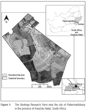
The study area was located in the Ukulinga Research Farm at the University of KwaZulu-Natal in Pietermaritzburg (30°24'S, 29°24'E) (Figure 1). The area is characterised by warm to hot summers and mild winters which often are accompanied by occasional frost. Mean monthly temperature ranges from 13.2 °C to 21.4 °C, with an annual mean of 17 °C.^31,32 The farm receives over 106 days of rain with an annual precipitation of about 680 mm. Soils originate from shallow marine shales of Lower Permian Ecca Group classified as Westleigh forms. The area is under the Southern Tall Grassveld and is predominately herbaceous as a result of frequent mowing and long-term burnings.³²Themeda triandra Forssk, Heteropogon contortus (L.) P Beauv. ex Roem. Schult. and Tristachya leucothrix Trin. ex Nees dominate the area.³³

 

 

Field sampling

Data were collected during the southern hemisphere summer (October 2014 to March 2015). Stratified random sampling with clustering was adopted to select sampling sites. The grassland area was first digitised from an aerial photograph (Figure 1) and stratified into north, south, east and west aspects. To select the plots, 10 x-y coordinates were randomly generated from the stratum using the Hawth tool. In total, 40 plots (30 m x 30 m) were selected and located in the field using a GPS (Trimple GEO XT with an estimated 100-mm accuracy). Two or three subplots of 1 m x 1 m were randomly chosen within each plot to generate a final sample size of 100 plots. Spectral and LAI data were then collected within the subplots at the onset of, mid- and end of summer.

Data collection

At each sampling point, LAI was acquired with a LAI-2200C Plant Canopy Analyzer using the procedure described by Darvishzadeh et al.⁷ Canopy reflectance was acquired using an analytical spectral device (ASD FieldSpec® 3 spectrometer, Boulder, CO, USA). The spectral resolution of the ASD FieldSpec® 3 spectrometer ranges from 350 nm to 2500 nm with 1.4-nm and 2-nm sampling intervals for the ultraviolet to visible and NIR region (350-1000 nm) and the SWIR region (1000-2500 nm) respectively. To normalise the spectra collected, the radiance of a white standard panel coated with barium sulfate and of known reflectivity was first recorded. Canopy reflectance measurements were made under clear sky between 10:00 and 14:00 local time to minimise atmospheric effects. To account for any changes in the atmospheric condition and the sun irradiance, reflectance measurements were recorded with frequent normalisation using the standard panel.³⁴ In total, 15 replicates of canopy reflectance within each subplot were collected and averaged, allowing for elimination of measurement noise arising from soil background.⁷

Data analysis

Pre-processing of hyperspectral data

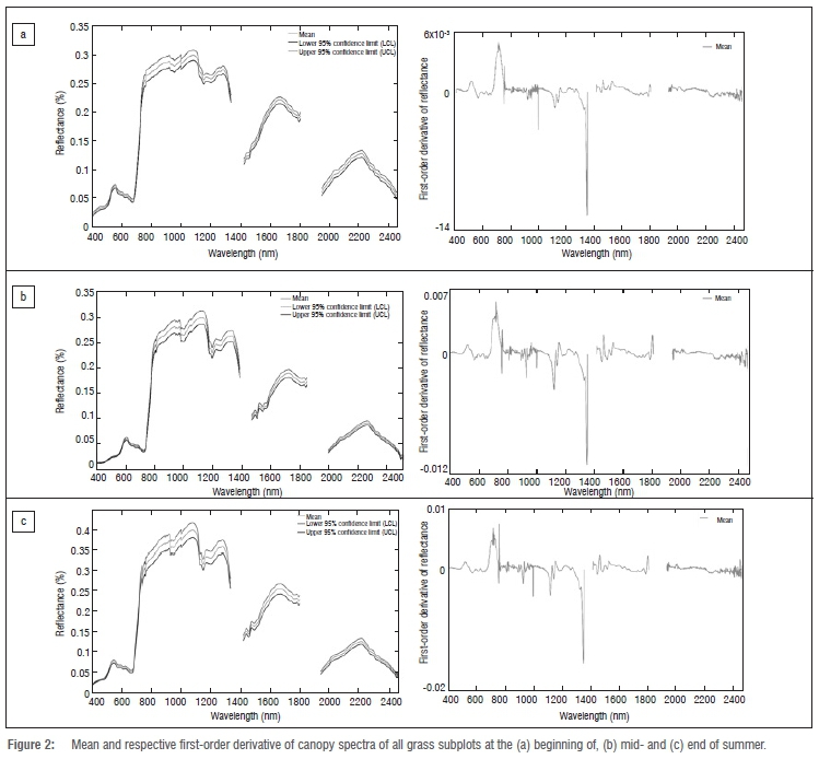
To separate overlapping bands, thereby amplifying fine differences in the electromagnetic spectrum, the first-order derivative at three nanometres was applied on the resulting mean spectral data.^35,36 First-order derivative is also known to be useful in minimising atmospheric and background noise.^14,20 A number of researchers^7,37,38 have applied first-order derivative on hyperspectral data for LAI estimation. The spectral regions of 350-399 nm, 1355-1420 nm, 1810-1940 nm and 2470-2500 nm (Figure 2) are known to be noisy and were discarded from the spectra.^5,39

Analysis of variance and Brown-Forsythe tests

The combined test of skewness and kurtosis was first employed to evaluate the distribution of the collected LAI data. The test of normality is a prerequisite to assessing data variability. A perfect normal distribution has skewness and kurtosis values equal to zero.⁴⁰ To assess LAI variations between periods within summer, one-way analysis of variance (ANOVA) and Brown-Forsythe tests (α=0.05) were implemented. The use of the Brown-Forsythe test, in addition to ANOVA, was justified by the smaller sample size at the end of summer (n=73) because of spectrometer failure. According to Maxwell and Delaney⁴¹ and Sheskin⁴², the Brown-Forsythe test is preferred over ANOVA when sample sizes are heterogeneous and is less affected by data that are not normally distributed.

Partial least squares regression

Partial least squares regression was originally an econometric technique created by Herman Wold in the 1960s to construct predictive models from highly collinear explanatory variables.²⁵ The principle of PLSR is to firstly decompose explanatory variables (X) into a few non-correlated latent variables or components using information contained in the response variable (Y); then to regress the new components against the response variable.^23,43 According to Tan and Li⁴⁴, Wang et al.⁴⁵ and Yeniay and Goktas²⁵, the model that underlies PLSR consists of three phases. In the first phase, explanatory (X) and response (Y) variables are decomposed based on the expression:

where T and U are respective matrices of scores of X and Y; P and Q stand for the matrices of loadings; and E and F for errors of X and Y matrices. In the second phase, the Y-scores (U) are predicted using the X-scores (T) based on the expression:

where b represents the regression coefficient and e the error matric of the relationship between Y-scores and X-scores. In the final phase, the predicted Y-scores are used to build predictive models of response variable using the expression:

where G is the error matrix related to estimating Y

In the present study, we used the PLS Toolbox (Eigenvector Research Inc.) with MATLAB (version R2013b) to build PLSR models. Before running PLSR, pre-processed hyperspectral data along with LAI data were autoscaled.¹¹ This procedure scales mean-centres of each waveband to unit standard deviation.⁴⁶ The PLSR was then run on data using a leave-one-out cross-validation method. The least root mean square error (RMSE) and the highest coefficients of determination (R²) between the predicted and the measured Y variable were the two criteria used to select the best model with optimal number of components. The best model was suggested by the software.

Interval partial least squares regression

Interval partial least squares regression (iPLSR) is a variant of PLS that locally develops PLS models on equidistant portions of the full spectrum.^26,27 To predict a Y variable from spectra using iPLSR, the spectrum is split into a number of intervals of equal distance. A PLSR model is then built on each spectral interval. Thereafter, all the models built on the wavebands of different intervals are compared to the full-spectrum model based on calibration parameters such as root mean square error of cross-validation (RMSECV). Finally, the local model with the lowest RMSECV is selected.^21,47 The iPLSR can operate in two modes or variable selection directions: backward and forward mode. In forward mode, the algorithm starts without any variable selection and then develops the best PLSR model from the interval with the lowest RMSECV. This process can be repeated by including more intervals to enhance the model. In backward mode, the algorithm starts by selecting all variables and then discards the interval with the largest RMSECV.⁴⁸

In this study, iPLSR in forward mode was used to select best spectral intervals. As predictive bands of LAI are known to spread across the entire electromagnetic spectrum as mentioned above, the interval size was set to a single variable. This approach is recommended when there is uniqueness of information in variables.⁴⁶ After several adjustments, the process was repeated 40 times. Therefore, the output local model had 40 intervals or bands. The iPLSR in forward mode was implemented using the PLS Toolbox.

Validation

A leave-one-out cross-validation method was implemented to calibrate models using 70% of the data and to find the optimal number of components. Then, the performance of trained models was validated using 30% of the data (independent data set). To assess model performance for prediction at the three sampling periods, relative root mean square regression to the mean (nRMSEP) and coefficient of determination (R²_P) were used.

Data splitting into training and independent test data sets was performed using an onion algorithm.⁴³ An onion algorithm was chosen in this study to avoid arbitrary data splitting which may cause biased results.⁷ The principle of onion algorithm is to keep outside covariant data plus those that are randomly inner spaced.⁴⁹

 

Results

Variation in LAI and spectra data

The values of skewness (between 0.40 and -0.45) and kurtosis (between 0.86 and -0.11) indicate that the LAI of grass species canopy in the sampling plots had a normal distribution. Therefore the LAI data were suitable for the ANOVA and Brown-Forsythe tests. LAI variation in grass species canopy was significant among the three multi-temporal periods (p<0.01). Samples in mid-summer had the highest mean (3.63 m²/m²) and variability (standard deviation= 1.10 m²/m²). Samples at the end of summer had the second highest mean (2.01 m²/m²) and lowest variability (standard deviation = 0.705 m²/m²). Samples at the beginning of summer had the least mean value of LAI (1.667 m²/m²) in grass species canopies, with the second least variability (0.821 m²/m²) in LAI.

To assess the change in reflectance at the different sampling periods, the mean spectra of all the sampling plots were averaged and upper and lower 95% confidence limits were derived. Results show that there was a change in averaged reflectance during the sampling periods (Figure 2). Visually, averaged reflectance was noticeably different across the electromagnetic spectrum. Canopy reflectance at the end, beginning and mid-summer presented the highest mean reflectance in the visible, NIR and SWIR regions, respectively. Figure 2 shows that first-derivative spectra differed in some spectral portions at the different sampling periods. The highest values of first-order derivative of reflectance are located in the NIR and SWIR region of the electromagnetic spectrum.

PLSR and iPLSR models

Table 1 presents results of the model performance of PLSR and iPLSR for the training data set at each of the sampling periods within summer. Based on RMSECV and R², results show that the iPLSR models perform better than the PLSR models. At each period, iPLSR models were able to explain more than 85% of LAI variability (88.8% at the beginning, 90.3% of mid- and 89.6% at the end of summer) with RMSECV values that vary from 0.24 m²/m² to 0.32 m²/m². Although iPLSR had a slightly higher RMSECV value (0.53 m²/m²) it had a better estimation of LAI variability across the entire summer (R²_cv = 0.81). PLSR models on the other hand yielded high RMSECV values (0.55-0.77 m²/m²) and poorly explained the LAI variation (31.3-67.1%).

 

 

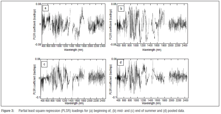
The contribution of each waveband in the selected PLSR factors is displayed in Figure 3. The most valuable bands for estimating LAI were distributed across the electromagnetic spectrum. However, the highest peaks for all the periods within summer, including all the periods combined, were mostly located in the NIR and SWIR regions.

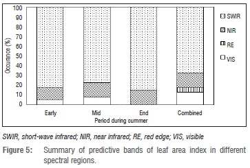
Using iPLSR models with 40 intervals, Table 2 and Figure 4 present the selected bands and their location within the four regions of the electromagnetic spectrum, respectively, while Figure 5 provides a percentage of predictive bands in relation to the regions within the electromagnetic spectrum.

 

 

Model validation

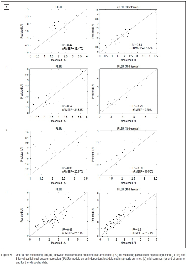
Figure 6 shows the performance of PLSR and iPLSR (40 intervals) models on the independent test data set. PLSR models of all the periods within summer (including all the periods combined) increased the coefficient of determination for prediction (R²_p) and slightly decreased the relative root mean square error for prediction (nRMSEP). The values of R²_p and nRMSEP respectively, varied from 0.36 to 0.65 and from 28.44% (0.69 m²/m²) to 33.47% (0.56 m²/m²). However, iPLSR models performed better than the full-spectrum PLRS models for all the sampling periods in summer. The predictive power of iPLSR models did not change much on the validation data set. More than 80% of new data of LAI could be explained by the iPLSR models at all periods within summer (including all the periods combined).

 

Discussion

We sought to determine the performance of two multivariate regression models (PLSR and iPLSR) in estimating canopy level LAI on tropical grassland during summer. Comparisons were determined using the coefficient of determination (R²) and the RMSE. Specifically, we examined the possibility of developing a model that can estimate LAI at different periods within summer (beginning, mid- and end) and across the entire summer period. Use of iPLSR to select the optimal bands for predicting LAI was also investigated.

Results showed that the PLSR algorithm run on first-derivative spectra to assess LAI variation at different periods did not perform well. The values of R²_p and nRMSEP, respectively, ranged from 0.36 to 0.65 and 34.53% to 28.44%. Although PLSR is known to reduce the dimensionality of data to a few uncorrelated (orthogonal) components, inclusion of all the wavebands was not useful in the predictive performance of PLSR models - results consistent with Liu⁵⁰, Chung and Keles⁵¹ and Filzmoser et al.⁵² However, when data dimensionality was reduced to useful bands using iPLSR, the performance of models (R² and RMSE) significantly improved. Overall, there were very close relationships between measured and predicted LAI values, with low values of RMSE and higher values of determination coefficients (R²) (Figure 6). Consistent with the findings of Zou et al.⁵³, Norgaard et al.²⁶ and Navea et al.²⁷, our findings confirm the superiority of iPLSR over full-spectrum PLSR.

The best predictive performance was derived from canopy reflectance at mid- (R²_p = 0.93 and nRMSEP = 9.39%) and end summer (R²_p = 0.89 and nRMSEP = 10.50%). The models performed the worst at the beginning of summer (R²_p = 0.88 and nRMSEP = 17.37%) and for all the sampling periods combined (R²_p = 0.81 and nRMSEP = 24.71%). The lower early summer prediction in comparison to the two other sampling periods can be attributed to higher soil background noise. According to Darvishzadeh et al.⁷, soil background often has a negative effect on the predictive power of hyperspectral data when LAI is low. The lower performance at the end of summer in comparison to mid-summer might also be caused by soil background reflectance emanating from litters.

Adoption of iPLSR was useful in identifying relevant wavebands for predicting LAI. In total, 40 intervals were identified for all the sampling periods. The success of iPLSR for band selection in this study may be attributed to successful separation of overlapping bands performed by the first-derivative technique on the spectra. The spectral regions (NIR and SWIR) of bands selected by iPLSR are consistent with the findings by Darvishzadeh et al.⁷, Thenkabail et al.³⁸, Brown et al.⁵⁴ and Gong et al.⁵⁵ Within ±12 nm, the bands chosen (Figure 4) in this study showed a consistency with the known bands for estimating LAI. For example, bands near 793 nm, 1061 nm, 1062 nm, 1633 nm, 442 nm, 443 nm, 535 nm, 551 nm, 732 nm and 2190 nm were also identified by Wang et al.³⁷ for estimating rice LAI at different growth phases. Furthermore, Gong et al.⁵⁵ found that bands centred near 1201 nm, 1240 nm, 1062 nm, 1640 nm, 2097 nm and 2259 nm were useful for estimating forest LAI.

It is worth noting that the contribution of different spectral regions along with their wavebands to LAI estimation depends on a particular period within summer (Figure 4). This dependence might be explained by the fact that the positions of selected wavebands are sensitive to changes in LAI, as indicated by ANOVA and Brown-Forsythe test results. Thus, the positions vary when factors like biochemical (e.g. chlorophyll) and biophysical (e.g. canopy closure) parameters and background effects change with canopy growth phases.³⁷ For example, at the end of summer, as the canopy senesces and the amount of chlorophyll declines, NIR and SWIR become more important in predicting LAI.²⁸ Furthermore, in the combined period, the selected bands can be explained by the fact that they were insensitive to changes in LAI (see Table 2). Delegido et al.⁵⁶ found that vegetation indices combining bands at 674 nm and 712 nm could overcome the aforementioned saturation problem while Kim et al.⁵⁷ found similar results with the ratio of 550 nm and 700 nm, which were insensitive to changes in chlorophyll concentration.

In this study, iPLSR models have proved to outperform full-spectrum PLSR models. However, model performance has shown to depend on the period within summer, on vegetation and on site conditions. These limitations are expected because PLSR and its variants (e.g. iPLSR), which are linear regression techniques, empirically relate to LAI and spectral reflectance, which makes the models non-transferable when environmental conditions of grassland (or vegetation cover in general) change.²⁴ Further work should look at comparing iPLSR with other robust and flexible methods, such as physically based radiative transfer models, particularly for the combined period. Models for the combined period used physical laws to explicitly relate biophysical variables and spectral variation of canopy reflectance. Consequently, these models are known to be more reproducible than linear regression models such as PLSR.⁵⁸ Currently, rapid development is being undertaken on physically based radiative transfer models for application in the field of remote sensing.⁵⁹ Further studies should also compare iPLSR with non-linear machine learning (e.g. random forest, support vector machine) techniques as they are able to cope with non-linear relationships between biophysical variables and canopy reflectance in dense grasslands.⁶⁰

 

Conclusions

The following conclusions can be drawn:

• iPLSR can be used to simplify the relationship between LAI and canopy reflectance transformed using first-derivative technique better than PLSR can. The best iPLSR relationship is at the beginning and end of summer.
• By including all the variables, full-spectrum PLSR models yield a higher prediction error.
• iPLSR used as a single variable selection algorithm for LAI estimation can generate stable and reliable models with 40 bands.
• The period within summer, which is associated with vegetation growth, determines the selection and accuracy of LAI predictive bands.

Results show that appropriate band selection on in-situ hyperspectral data using iPLSR can overcome the challenge faced by remotely sensed data to accurately estimate LAI in a heterogeneous grassland. The findings pave the way to more accurate mapping and monitoring of canopy characteristics in a tropical grassland from airborne and space-borne hyperspectral data. However, the development of a iPLSR model for all the periods combined within summer needs further investigation, as its prediction error was higher than those for the periods separately.

 

Acknowledgements

We thank Brice Gijsbertsen and Victor Bangamwabo for technical support. We thank the Eigenvector Research Inc. for the free software PLS Toolbox. We also are grateful to Ognelet Marie Claude for his financial support throughout the life cycle of this research. Lastly, we acknowledge fellow students Dube Thimothy and Mfundiso Cele for their field assistance and the anonymous reviewers for improving the quality of this paper.

Authors' contributions

Z.K. was responsible for the data analysis and write-up; J.O. and O.M. edited and revised the manuscript.

 

References

1. He Y Guo X, Wilmshurst JF. Comparison of different methods for measuring leaf area index in a mixed grassland. Can J Plant Sci. 2007;87(4):803-813. https://doi.org/10.4141/CJPS07024        [ Links ]

2. Prins HHT, Beekman JH. A balanced diet as a goal for grazing - the food of the manyara buffalo. Afr J Ecol. 1989;27(3):241-259. https://doi.org/10.1111/j.1365-2028.1989.tb01017.x        [ Links ]

3. Broge NH, Mortensen JV. Deriving green crop area index and canopy chlorophyll density of winter wheat from spectral reflectance data. Remote Sens Environ. 2002;81(1):45-57. https://doi.org/10.1016/S0034-4257(01)00332-7        [ Links ]

4. Chen JM, Cihlar J. Retrieving leaf area index of boreal conifer forests using Landsat TM images. Remote Sens Environ. 1996;55(2):153-162. https://doi.org/10.1016/0034-4257(95)00195-6        [ Links ]

5. Abdel-Rahman EM, Mutanga O, Odindi J, Adam E, Odindo A, Ismail R. A comparison of partial least squares (PLS) and sparse PLS regressions for predicting yield of Swiss chard grown under different irrigation water sources using hyperspectral data. Comput Electron Agric. 2014;106:11-19. https://doi.org/10.1016/j.compag.2014.05.001        [ Links ]

6. Breda NJJ. Ground-based measurements of leaf area index: A review of methods, instruments and current controversies. J Exp Bot. 2003;54(392):2403-2417. https://doi.org/10.1093/jxb/erg263        [ Links ]

7. Darvishzadeh R, Skidmore A, Schlerf M, Atzberger C, Corsi F, Cho M. LAI and chlorophyll estimation for a heterogeneous grassland using hyperspectral measurements. ISPRS J Photogramm Remote Sens. 2008;63(4):409-426. https://doi.org/10.1016/j.isprsjprs.2008.01.001        [ Links ]

8. Shen L, Li Z, Guo X. Remote sensing of leaf area index (LAI) and a spatiotemporally parameterized model for mixed grasslands. Int J Appl. 2014;4(1):46-61.         [ Links ]

9. Xu LK, Baldocchi DD. Seasonal variation in carbon dioxide exchange over a Mediterranean annual grassland in California. Agric For Meteorol. 2004;123(1-2):79-96. https://doi.org/10.1016/j.agrformet.2003.10.004        [ Links ]

10. Jonckheere I, Fleck S, Nackaerts K, Muys B, Coppin P Weiss M, et al. Review of methods for in situ leaf area index determination - Part I. Theories, sensors and hemispherical photography. Agric For Meteorol. 2004;121(1-2):19-35. https://doi.org/10.1016/j.agrformet.2003.08.027        [ Links ]

11. Zhang R, Ba J, Ma Y Wang S, Zhang J, Li W, editors. A comparative study on wheat leaf area index by different measurement methods. Proceedings of the First International Conference on Agro-Geoinformatics; 2012 August 2-4: Shangai, China. IEEE; 2012. https://doi.org/10.1109/Agro-Geoinformatics.2012.6311671        [ Links ]

12. Chason JW, Baldocchi DD, Huston MA. A comparison of direct and indirect methods for estimating forest canopy leaf-area. Agric For Meteorol. 1991;57(1-3):107-128. https://doi.org/10.1016/0168-1923(91)90081-Z        [ Links ]

13. Bulcock HH, Jewitt GPW. Spatial mapping of leaf area index using hyperspectral remote sensing for hydrological applications with a particular focus on canopy interception. Hydrol Earth Syst Sci. 2010;14(2):383-392. https://doi.org/10.5194/hess-14-383-2010        [ Links ]

14. Pullanagari RR, Yule IJ, Tuohy MP Hedley MJ, Dynes RA, King WM. Infield hyperspectral proximal sensing for estimating quality parameters of mixed pasture. Precis Agric. 2012;13(3):351-369. https://doi.org/10.1007/s11119-011-9251-4        [ Links ]

15. Atzberger C, Jarmer T, Schlerf M, Kotz B, Werner W, editors. Spectroradiometric determination of wheat bio-physical variables. Comparison of different empirical-statistical approaches. In: Remote Sensing in Transition; 2003 June 2-5; Ghent, Belgium. Rotterdam: Millpress; 2004. Available from: http://www.geo.uzh.ch/microsite/rsl-documents/research/publications/other-sci-communications/Atzberger_etal_Gent2003-2987622144/Atzberger_etal_Gent2003.pdf        [ Links ]

16. Hansen P Schjoerring J. Reflectance measurement of canopy biomass and nitrogen status in wheat crops using normalized difference vegetation indices and partial least squares regression. Remote Sens Environ. 2003;86(4):542-553. https://doi.org/10.1016/S0034-4257(03)00131-7        [ Links ]

17. Lee KS, Cohen WB, Kennedy RE, Maiersperger TK, Gower ST. Hyperspectral versus multispectral data for estimating leaf area index in four different biomes. Remote Sens Environ. 2004;91(3-4):508-520. https://doi.org/10.1016/j.rse.2004.04.010        [ Links ]

18. Li X, Zhang Y Bao Y Luo J, Jin X, Xu X, et al. Exploring the best hyperspectral features for LAI estimation using partial least squares regression. Remote Sens. 2014;6(7):6221-6241. https://doi.org/10.3390/rs6076221        [ Links ]

19. Nguyen HT, Lee BW. Assessment of rice leaf growth and nitrogen status by hyperspectral canopy reflectance and partial least square regression. Eur J Agron. 2006;24(4):349-356. https://doi.org/10.1016/j.eja.2006.01.001        [ Links ]

20. Dorigo WA, Zurita-Milla R, De Wit AJW, Brazile J, Singh R, Schaepman ME. A review on reflective remote sensing and data assimilation techniques for enhanced agroecosystem modeling. Int J Appl Earth Obs Geoinf. 2007;9(2):165-193. https://doi.org/10.1016/j.jag.2006.05.003        [ Links ]

21. Andersen CM, Bro R. Variable selection in regression-a tutorial. J Chemom. 2010;24(11-12):728-737. https://doi.org/10.1002/cem.1360        [ Links ]

22. Atzberger C, Guérif M, Baret F, Werner W. Comparative analysis of three chemometric techniques for the spectroradiometric assessment of canopy chlorophyll content in winter wheat. Comput Electron Agric. 2010;73(2):165-173. https://doi.org/10.1016/j.compag.2010.05.006        [ Links ]

23. Cho MA, Skidmore A, Corsi F, Van Wieren SE, Sobhan I. Estimation of green grass/herb biomass from airborne hyperspectral imagery using spectral indices and partial least squares regression. Int J Appl Earth Obs Geoinf. 2007;9(4):414-424. https://doi.org/10.1016/j.jag.2007.02.001        [ Links ]

24. Darvishzadeh R, Atzberger C, Skidmore A, Schlerf M. Mapping grassland leaf area index with airborne hyperspectral imagery: A comparison study of statistical approaches and inversion of radiative transfer models. ISPRS Int J Remote Sens. 2011;66(6):894-906. https://doi.org/10.1016/j.isprsjprs.2011.09.013        [ Links ]

25. Yeniay O, Goktas A. A comparison of partial least squares regression with other prediction methods. Hacet J Math Stat. 2002;31(99):99-101.         [ Links ]

26. Norgaard L, Saudland A, Wagner J, Nielsen JP Munck L, Engelsen SB. Interval partial least-squares regression (iPLS): A comparative chemometric study with an example from near-infrared spectroscopy. Appl Spectrosc. 2000;54(3):413-419. https://doi.org/10.1366/0003702001949500        [ Links ]

27. Navea S, Tauler R, De Juan A. Application of the local regression method interval partial least-squares to the elucidation of protein secondary structure. Anal Biochem. 2005;336(2):231-242. https://doi.org/10.1016/j.ab.2004.10.016        [ Links ]

28. Zhao D, Huang L, Li J, Qi J. A comparative analysis of broadband and narrowband derived vegetation indices in predicting LAI and CCD of a cotton canopy. ISPRS J Photogramm Remote Sens. 2007;62(1):25-33. https://doi.org/10.1016/j.isprsjprs.2007.01.003        [ Links ]

29. Mutanga O, Skidmore AK. Narrow band vegetation indices overcome the saturation problem in biomass estimation. Int J Remote Sens. 2004;25(19):3999-l014. https://doi.org/10.1080/01431160310001654923        [ Links ]

30. Pu R, Gong P Biging GS, Larrieu MR. Extraction of red edge optical parameters from hyperion data for estimation of forest leaf area index. IEEE Transactions on Geoscience and Remote Sensing. 2003;41(4):916-921. https://doi.org/10.1109/TGRS.2003.813555        [ Links ]

31. Everson CS, Mengistu MG, Gush MB. A field assessment of the agronomic performance and water use of Jatropha curcas in South Africa. Biomass Bioenerg. 2013;59:59-69. https://doi.org/10.1016/j.biombioe.2012.03.013        [ Links ]

32. Mills AJ, Fey MV. Frequent fires intensify soil crusting: Physicochemical feedback in the pedoderm of long-term burn experiments in South Africa. Geoderma. 2004;121(1-2):45-64. https://doi.org/10.1016/j.geoderma.2003.10.004        [ Links ]

33. Ghebrehiwot HM, Kulkarni MG, Szalai G, Soos V Balazs E, Van Staden J. Karrikinolide residues in grassland soils following fire: Implications on germination activity. S Afr J Bot. 2013;88:419-424. https://doi.org/10.1016/j.sajb.2013.09.008        [ Links ]

34. Rajah P Odindi J, Abdel-Rahman EM, Mutanga O, Modi A. Varietal discrimination of common dry bean (Phaseolus vulgaris L.) grown under different watering regimes using multi-temporal hyperspectral data. J Appl Remote Sensing. 2015;9(1):096050-096050.         [ Links ]

35. Archontaki HA, Atamian K, Panderi IE, Gikas EE. Kinetic study on the acidic hydrolysis of lorazepam by a zero-crossing first-order derivative UV-spectrophotometric technique. Talanta. 1999;48(3):685-693. https://doi.org/10.1016/S0039-9140(98)00288-4        [ Links ]

36. Holden H, LeDrew E. Spectral discrimination of healthy and non-healthy corals based on cluster analysis, principal components analysis, and derivative spectroscopy. Remote Sens Environ. 1998;65(2):217-224. https://doi.org/10.1016/S0034-4257(98)00029-7        [ Links ]

37. Wang F-m, Huang J-f, Zhou Q-f, Wang X-z. Optimal waveband identification for estimation of leaf area index of paddy rice. J Zhejiang Univ Sci B. 2008;9(12):953-963. https://doi.org/10.1631/jzus.B0820211        [ Links ]

38. Thenkabail PS, Enclona EA, Ashton MS, Van der Meer B. Accuracy assessments of hyperspectral waveband performance for vegetation analysis applications. Remote Sens Environ. 2004;91(3-4):354-376. https://doi.org/10.1016/j.rse.2004.03.013        [ Links ]

39. Adjorlolo C, Mutanga O, Cho MA, Ismail R. Spectral resampling based on user-defined inter-band correlation filter: C3 and C4 grass species classification. Int. J Appl Earth Obs. Geoinf. 2013;21:535-544. https://doi.org/10.1016/j.jag.2012.07.011        [ Links ]

40. Peat J, Barton B. Medical statistics: A guide to data analysis and critical appraisal. Malden, MA: Blackwell Publishing; 2005. https://doi.org/10.1002/9780470755945        [ Links ]

41. Maxwell SE, Delaney HD. Designing experiments and analyzing data: A model comparison perspective. 2nd ed. New York: Psychology Press; 2004.         [ Links ]

42. Sheskin DJ. Handbook of parametric and nonparametric statistical procedures. Boca Raton, FL: Chapman and Hall/CRC; 2011.         [ Links ]

43. Tobias RD, editor. An introduction to partial least squares regression. Paper presented at: Twentieth Annual SAS Users Group International conference; 1995 April 2-5; Orlando, Florida, USA.         [ Links ]

44. Tan C, Li M. Mutual information-induced interval selection combined with kernel partial least squares for near-infrared spectral calibration. Acta Mol Biomol Spectrosc. 2008;71(4):1266-1273. https://doi.org/10.1016/j.saa.2008.03.033        [ Links ]

45. Wang F-m, Huang J-f, Lou Z-h. A comparison of three methods for estimating leaf area index of paddy rice from optimal hyperspectral bands. Precis Agric. 2011;12(3):439-447. https://doi.org/10.1007/s11119-010-9185-2        [ Links ]

46. Wise BM, Gallagher NB, Bro R, Shaver JM, Windig W, Koch RS. PLS_Toolbox version 4.0 for use with MATLAB™. Manson, WA: Eigenvector; 2006        [ Links ]

47. Bezerra de Lira LF, De Albuquerque MS, Andrade Pacheco JG, Fonseca TM, De Siqueira Cavalcanti EH, Stragevitch L, et al. Infrared spectroscopy and multivariate calibration to monitor stability quality parameters of biodiesel. Microchem J. 2010;96(1):126-131. https://doi.org/10.1016/j.microc.2010.02.014        [ Links ]

48. Mehmood T, Liland KH, Snipen L, Saebo S. A review of variable selection methods in partial least squares regression. Chemometr Intell Lab. 2012;118:62-69. https://doi.org/10.1016/j.chemolab.2012.07.010        [ Links ]

49. Sousa AG, Ahl LI, Pedersen HL, Fangel JU, Sorensen SO, Willats WGT. A multivariate approach for high throughput pectin profiling by combining glycan microarrays with monoclonal antibodies. Carbohydr Res. 2015;409:41-47. https://doi.org/10.1016/j.carres.2015.03.015        [ Links ]

50. Liu J. Developing a soft sensor based on sparse partial least squares with variable selection. J Process Contr. 2014;24(7):1046-1056. https://doi.org/10.1016/j.jprocont.2014.05.014        [ Links ]

51. Chung D, Keles S. Sparse partial least squares classification for high dimensional data. Stat Appl Genet Mol. 2010;9(1), Art. #1492. https://doi.org/10.2202/1544-6115.1492        [ Links ]

52. Filzmoser P Gschwandtner M, Todorov V. Review of sparse methods in regression and classification with application to chemometrics. J Chemom. 2012;26(3-4):42-51. https://doi.org/10.1002/cem.1418        [ Links ]

53. Zou X, Zhao J, Huang X, Li Y. Use of FT-NIR spectrometry in non-invasive measurements of soluble solid contents (SSC) of 'Fuji' apple based on different PLS models. Chemometr Intell. 2007;87(1):43-51. https://doi.org/10.1016/j.chemolab.2006.09.003        [ Links ]

54. Brown L, Chen JM, Leblanc SG, Cihlar J. A shortwave infrared modification to the simple ratio for LAI retrieval in boreal forests: An image and model analysis. Remote Sens Environ. 2000;71(1):16-25. https://doi.org/10.1016/S0034-4257(99)00035-8        [ Links ]

55. Gong P, Pu RL, Biging GS, Larrieu MR. Estimation of forest leaf area index using vegetation indices derived from Hyperion hyperspectral data. IEEE Trans Geosci Remote Sens. 2003;41(6):1355-1362. https://doi.org/10.1109/TGRS.2003.812910        [ Links ]

56. Delegido J, Verrelst J, Meza CM, Rivera JP, Alonso L, Moreno J. A red-edge spectral index for remote sensing estimation of green LAI over agroecosystems. Eur J Agron. 2013;46:42-52. https://doi.org/10.1016/j.eja.2012.12.001        [ Links ]

57. Kim MS, Daughtry CST, Chappelle EW, Mcmurtrey JE, Walthall CL, editors. The use of high spectral resolution bands for estimating absorbed photosynthetically active radiation (A par). In: CNES, Proceedings of 6th International Symposium on Physical Measurements and Signatures in Remote Sensing; 1994; Val D'Isere, France. Val D'Isere: The Symposium, 1994. p. 299-306.         [ Links ]

58. Quan X, He B, Yebra M, Yin C, Liao Z, Zhang X, et al. A radiative transfer model-based method for the estimation of grassland aboveground biomass. Int J Appl Earth Obs Geoinf. 2017;54:159-168. https://doi.org/10.1016/j.jag.2016.10.002        [ Links ]

59. Jacquemoud S, Verhoef W, Baret F, Bacour C, Zarco-Tejada PJ, Asner GP, et al. PROSPECT+ SAIL models: A review of use for vegetation characterization. Remote Sens Environ. 2009;113:S56-S66. https://doi.org/10.1016/j.rse.2008.01.026        [ Links ]

60. Kiala Z, Odindi J, Mutanga O, Peerbhay K. Comparison of partial least squares and support vector regressions for predicting leaf area index on a tropical grassland using hyperspectral data. J Appl Remote Sens. 2016;10(3), Art. #036015, 14 pages. https://doi.org/10.1117/1.JRS.10.036015        [ Links ]

 

 

Correspondence:
Zolo Kiala
serkial1@yahoo.fr

Received: 08 Sep. 2016
Revised: 18 Jan. 2017
Accepted: 09 May 2017