RESEARCH ARTICLE

 

Extreme 1-day rainfall distributions: Analysing change in the Western Cape

 

 

Jan H. de Waal^I; Arthur Chapman^II; Jaco Kemp^I

^IDepartment of Geography and Environmental Studies, Stellenbosch University, Stellenbosch, South Africa
^IIPrivate consultant, Jonkershoek, Stellenbosch, South Africa

Correspondence

 

 

---

ABSTRACT

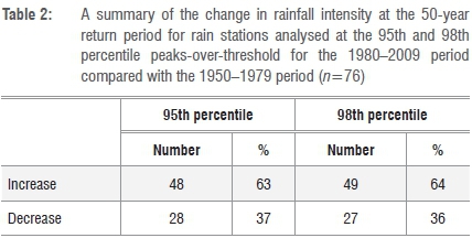
Severe floods in the Western Cape Province of South Africa have caused significant damage to property and infrastructure over the past decade (2003-2014). The hydrological design criteria for exposed structures and design flood calculations are based mostly on the implicit assumption of stationarity, which holds that natural systems vary within an envelope of variability that does not change with time. This assumption was tested by examining the changes in extreme 1-day rainfall high percentiles (95th and 98th) and both the 20- and 50-year return period rainfall, comparing the period 1950-1979 against that of 1980-2009 across the province. A generalised Pareto distribution and a peaks-over-threshold sampling approach was applied to 76 rainfall stations across the province. Of these stations, 48 (63%) showed an increase in the 50-year return period 1-day rainfall and 28 (37%) showed a decrease in the 1980-2009 period at the 95th percentile peaks-over-threshold. At the 98th percentile peaks-over-threshold, 49 stations (64%) observed an increase and 27 (36%) a decrease for the later period. The change in the number of 3-day storms from the first to the second period is negligible, evaluated at 0.9% and 0.5% at the 95th and 98th percentile peaks-over-threshold levels, using cluster analysis. While there is no clear spatial coherency to the results, the general trend indicates an increase in frequency of intense rainfalls in the latter half of the 20th and early 21st centuries. These results bring into question assumptions of stationarity commonly used in design rainfall.
SIGNIFICANCE:
•63% of analysed rainfall stations in the Western Cape display an increase in 20- and 50-year 1-day rainfall extremes.
•The results challenge the current assumptions of climate stationarity made in design rainfall estimations.
•We propose an alternative methodology to rainfall extremes analysis for design flood estimation.
•The methods employed can be replicated by future studies in other regions.

Keywords: extreme rainfall; stationarity; hazard; climate; generalised Pareto distribution

---

 

 

Introduction

Katz et al.¹ state that 'it is the unusual disturbances that have disproportionate effects on ecosystems'. This view can be extended to economic infrastructure. From 2003 to 2014, the Western Cape Province of South Africa (Figure 1) has been affected by severe storms occurring almost annually, which cause substantial damage to economic infrastructure and farmlands.^2,3 These severe floods, caused mostly by intense rainfall resulting from cut-off low weather systems, resulted in damage equating to at least ZAR4.9 billion (Table 1).^2,3

Whether this damage arises as a result of changes in the frequency and intensity of extreme rainfall, or of human intrusion into hazardous areas and land-use change is unknown. Unfortunately, financial loss records are sparse prior to the initial analysis done by Holloway et al.², making analysis of prior losses difficult. However, extreme rainfalls are the predominant drivers of flood risk and concerns of increases in the frequency and/or intensity of extremes have been raised across the world.⁴

Although national and provincial roads as well as hydraulic structures are designed for appropriate design lives,⁵ the probabilistic estimation methods (through the use of the annual maximum series) of these design floods are based on the assumption of stationarity of the rainfall regime. Stationarity is a theory that natural systems vary within an envelope of variability that does not change with time. This is a foundational concept that is prevalent throughout hydrological engineering practice.⁶ However, flood levels for given return periods are known to be increasing in some places in the world⁷, and are possibly decreasing in other parts, which may be a result of changing rainfalls in these regions⁸. A limitation to the estimation of reasonably accurate return period rainfalls is that it requires long records (multi-decadal) of high-quality data.⁷ Unfortunately, in many areas, the length of the data record is limited and the possibility of a non-stationary climate is largely ignored.⁶ The design of hydraulic structures and determination of design flood-levels therefore assumes that weather events are independent outcomes of a stationary climate.⁶ It is, however, evident that the climate is changing in some places⁹ and that the concept of stationarity is no longer an appropriate assumption, which potentially renders the design capacity of hydraulic structures inappropriate for the evolving conditions. We examined the stationarity of rainfall extremes for the historical rainfall record of 76 rainfall stations in the Western Cape Province (Figure 1) and, using appropriate statistical analytical processes, tested whether change is indeed occurring.

 

Previous studies examining changes in South African rainfall

Various previous studies have been undertaken to investigate the changing frequency and intensity of extreme rainfalls in South Africa. Mason et al.¹⁰ found significant changes in rainfall over 70% of South Africa, except in parts of the winter rainfall region (the Western Cape) for two periods: 1931-1960 and 1961-1990. According to their analysis, the intensity of the 10-year rainfall events had increased by 10% over much of the country except in the northeast (Limpopo and Mpumalanga Lowveld and the eastern Highveld), northwest and the winter rainfall region (Western Cape). However, the density of the rain gauge network used in the study was low for those areas, indicating declines in maximum rainfall intensity.

Easterling et al.¹¹ found significant increases in heavy rainfall frequency over the thresholds of 25.4 mm and 50.8 mm for southwestern South Africa (the Western Cape) and parts of KwaZulu-Natal, respectively. The frequencies of these events were estimated to increase at 5.5% and 4.1% per decade, respectively. Richard et al.¹² discovered an increase in rainfall in the southeastern part of the country in a review of time series rainfall data, while Groisman et al.¹³ showed an increase in frequency of very heavy rainfalls between the periods 1901-1910 and 1931-1997 for most of South Africa for those rainfalls equal to or above the 99.7 percentile (the upper 0.3%). Their data set was spatially differentiated by blocks of about 50 km on a side with six or more rain gauges per block. Kruger¹⁴ found that changes in annual maximum 1-day rainfalls for the Western Cape above the 99th percentile are inconclusive for records ending in 2002. New et al.¹⁵, using similar methods, showed that there was a 'statistically significant increase in regionally averaged daily rainfall intensity and dry spell duration' from 1961 to 2000 across the southern African region, but that few trends at individual stations were statistically significant.

 

Methods and data

One of the most important tasks in analysing extremes is to choose the statistical basis for the calculation.¹⁶ There are two fundamental approaches used in extreme value theory: the 'block maxima' approach, used in the annual maximum series and the 'peaks-over-threshold' (POT) approach.¹⁶ The traditional approach to extreme value analysis in South African rainfall analyses has been to use the annual maximum series.^5,17,18 The block maxima approach relies on identifying the highest value for each year and fitting a distribution to the data, while the POT approach fits a distribution to all data points that exceed a defined threshold.¹⁶

The advantage of the block maxima approach is its relative simple application; however, this method results in a substantial loss of information resulting from discarding values that are less than but close to the maximum in each year. As Katz¹⁶ argues, this modelling approach may result in poorer return level estimates and the POT may be considered a more appropriate alternative.

In this study, we therefore used the POT approach to analyse the changes in extreme return period rainfalls for 76 rainfall stations across the Western Cape and compare two equal periods: 1950-1979 and 1980-2009. The periods were chosen to split the record into two equal lengths and incorporate the most recent data that the South African Weather Service (SAWS) would supply.

Peaks-over-threshold

The POT approach is based on the same principle as that of the partial duration series, which was developed as a way of avoiding problems associated with the block maxima approach.¹⁹ The POT approach is predicated on fitting any suitable probability distribution, such as a generalised Pareto distribution (GPD), to all data points exceeding a defined extreme threshold.²⁰ The benefit of this approach is the inclusion of more data, but it does have the drawback that the events being observed may not be fully independent, which is a requirement for modelling.¹⁶

The POT approach obtains extreme values of a data set X₁, X₂, ... ,X_n by considering the exceedances Y = X - t over a sufficiently high threshold t. According to extreme value theory, the distribution of the exceedances Y₁, Y₂, ... ,Y_Nt, where N_t is the number of exceedances above the threshold t, can be reasonably approximated by a GPD.²¹ The distribution function of the GPD is given by Equation 1:

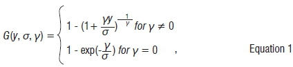
where σ and γ are the respective scale and shape parameters of the distribution. The shape parameter, which is known as the extreme value index in the generalised extreme value distribution, is considered the most important parameter in determining the tail behaviour of a distribution. The procedure of fitting the GPD to the exceedances above the threshold requires the estimation of the two unknown parameters σ and γ. Their maximum likelihood estimates can be obtained through maximisation of the log-likelihood function corresponding to the GPD,

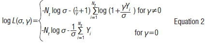
with respect to σ and γ.

This estimation task can be relatively easily executed using the function gpd.fit() available in the package ismev called by the statistical language R.²² The GPD is described as a heavy-tailed distribution, which is appropriate for rainfall analyses because extreme precipitation distributions largely exhibit heavy-tailed characteristics.^23-25

Use of the GPD requires a high threshold and the choice of threshold must be such that the excess over the threshold should have a nearly exponential distribution - to fit with the requirements of the GPD theorem.²⁶ A threshold value that is too large, however, will result in few data points (exceedances) from which the parameters of the GPD are estimated, with the consequence of possibly high variance of parameter and return level estimates. However, because the exceedances correspond to data points that lie far in the tail of the distribution of the original data, the limiting results on which the GPD is based are valid and the estimates are likely to exhibit low bias.²¹ In contrast, estimates that result from thresholds set too low will exhibit low variance as more data points (exceedances) are available for use in the estimation. However, data points that lie more towards the centre of the distribution of the original data, rather than in the tail, translate to estimates with higher degrees of bias.²¹ The choice of threshold is often made subjectively, keeping the above-mentioned bias-variance trade-off in mind.²¹ A statistical compromise needs to be achieved between setting the POT threshold high enough so that the excess distribution (above the threshold) converges to that of the GPD but low enough to have a sample of sufficient size so that the location, size and scale parameters can be estimated efficiently.²⁴

Setting the threshold high does not imply an exact value - the outcome is somewhat subjective. 'ismev' - an add-on package to the R statistical language - provides a technique of fitting a range of thresholds, in which the scale and shape parameters gradually change over the fitted range.²⁷ When setting the threshold, the scale and shape parameters should not end up diverging to such an extent as to imply increasing uncertainty in those parameters. While this is a useful process when applied as an intensive examination of an individual record, it is an overly time-consuming method when applied to many stations (as in this study). A more direct approach which could give sufficiently robust results is required. In similar extreme rainfall studies which evaluate many stations, two approaches are commonly adopted: (1) the use of relative thresholds or percentiles as thresholds (commonly the 95th and 98th percentiles) or (2) absolute thresholds.^4,28 We thus took two useful thresholds to be located at the 95th and 98th percentiles for each rainfall station. Separate thresholds at the 95th and 98th percentiles were estimated for each time period (1950-1979 and 1980-2009) as the two periods need to be viewed as separate data sets.

Cluster analysis

Rainfall exceedances over thresholds often occur in groups, with one extreme closely following another (because they may be caused by the same event) and this clustering produces dependence in the observations.²¹

In utilising the GPD function for deriving the probability distribution of rainfall events, it is assumed that rainfall extremes fit the Poisson process - a stochastic process in which events occur continuously (as opposed to discrete occurrences) and, importantly, independently of one another.¹⁶ The Poisson process has a long history of use in rainfall modelling.²⁹ It is therefore crucial to determine whether the data points that exceed the threshold value (threshold exceedances) are independent of each other when fitting a GPD.²⁴ This problem is addressed by making use of a process known as (de)clustering. Once a definition of cluster length of exceedances has been specified, only the maximum value in each cluster is retained and the remainder of the exceedances are discarded. This process then results in a 'new' set of exceedances that are approximately independent and the GPD can then be applied.

In the case of large storm systems such as cut-off low pressure systems, mid-latitude cyclones and cold fronts prevalent in the Western Cape, heavy rainfall can last for 3 days and more per storm. As a result, the observed rainfall may exceed the threshold value every day over a sequence of days for the same event and thus the individual daily observations may not be independent. These data points need to be 'declustered' in order to remove such related threshold exceedances.²¹ The process of declustering groups is done as another step with the 'evd' package, which has a specific function serving that purpose. In this study, a value of r=3 in the declustering process was considered reasonable. The value of the parameter implies that three consecutive threshold deficits following exceedances above the threshold indicate the end of a cluster. Further, in order to investigate the influence of cluster length on the results, r=2 and r=4 were also considered but showed very little variation in the outputs.

Following this definition of clusters of exceedances, a cluster can be interpreted as a single extreme 1-day rainfall event (the highest value).

Where:

n_t = the number of exceedances over the threshold t, and

n_c = the effective number of clusters.

The number of storms resulting in heavy rainfall lasting longer than a single day can be obtained by computing n_t - n_c. Here, n_c is referred to as the number of effective clusters rather than just the number of clusters, to emphasise that any cluster may consist of only a single exceedance above the threshold t. A GPD was then fitted to the new 'declustered' data set using the 'ismev' package in R.

Rainfall data

Rainfall stations used in this analysis were initially identified using the database compiled by Lynch³⁰. Suitably long (60 years - divided into two 30-year periods) records of daily rainfall data of SAWS stations were selected. The Lynch³⁰ data set terminates in 2001. SAWS supplied the remaining data to extend the records to 2009.

Long data records are required in order to divide the rainfall record into equal time periods and to have sufficient data points for the fitting of a distribution. Therefore, use was made of patched (infilled) data provided by the Lynch³⁰ data set.

The use of patched data for extreme value analysis has precedents in the literature^31,32 and we believe that it provides, in this research, an acceptable means for overcoming gaps in data and extending records where necessary, especially in the early parts of the records. The possible errors that could be introduced into the analysis using this method are low as the rainfall events have already been observed at nearby rain gauges. Although rainfall records extend further back than 1950 for all of the stations used, the quantity of infilled data in these records increases substantially for earlier patched data sets. Thus, rainfall stations were chosen based not only on data length, but also on the low totals of infilled data. The quantum of all exceedances greater than the 95th percentile of the data used in this study that are infilled is 1.4%.

Rainfall catch anomalies and inhomogeneities

Mason et al.¹⁰ and Zang et al.³³ mention the problem of inhomogeneities in the data. These inhomogeneities arise when a rain gauge is moved or instrumentation is changed, or as a result of other environmental factors that may influence rainfall catch. These authors caution against use of data containing inhomogeneities, noting that testing of long-term change requires quality-controlled data. Indeed, Mason et al.¹⁰ left out many gauges for potential analysis because of these perceptions.

We take a different view. Our approach is that the quantum of individual extreme 1-day rainfalls overwhelms subtle changes within a station time series, and that removing such data from the study implies an a priori understanding of the impacts of the inhomogeneities in the data on extreme values. Inhomogeneities in the extremes of temperature data, by contrast and comparison, are of real concern,³⁴ but are likely because temperature extremes - both maxima and minima - are far more strongly bounded in nature than precipitation extremes. Thus, measuring an extreme temperature of 51 °C is very unlikely under natural conditions (i.e. above a vegetated surface) and the probability of an extreme temperature of 52 °C above the same surface would decrease by an order of magnitude or more. Measuring a temperature of 60 °C is almost impossible under current circumstances (an increase from 51 °C of 17.6%). However, a comparison of two extremes of rainfall - e.g. 150 mm and 200 mm in 24 h, an increase of 33% - is quite plausible and the upper limit of rainfall is very poorly defined, for example 597 mm in one day was recorded at St Lucia during Cyclone Domoina on 31 January 1984.³⁵ Further, much of the data utilised in this study have already been checked and corrected for errors by Lynch³⁰.

 

Results and discussion

Two key results based on the 95th and 98th percentile POT sampling are presented here, in which there is a strong change to more frequent extreme 1-day rainfalls in the later part of the rainfall record. Both results are considered in more detail below in separate sections. However, a spatial representation of these results reveals that these changes do not provide a clear spatial pattern of change. A pattern may be evident but is difficult to determine because of the low station density across the province.

Changes in design rainfalls

Table 2 presents a summary of the changes in the 50-year return period rainfalls.

 

 

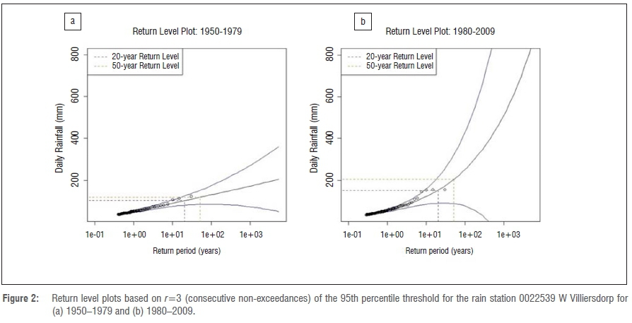
The GPD output is displayed in the return period rainfall plots in Figure 2 as examples. For the study, similar graphs were produced for each of the 76 rainfall stations. These graphs display the return period rainfalls (on the linear y-axis) against the return period (on the logarithmic x-axis) for both time periods.

The blue response functions (continuous curves) in Figure 2 indicate 95% confidence intervals, while the black response function is the curve indicating estimated return period rainfalls for the same periods. Figure 2 displays results for a rainfall station at Villiersdorp that had an increase in the 50-year return period rainfall magnitude from 118.2 mm for the period 1950-1979 to 202.6 mm for the period 1980-2009 - an increase of 71%.

It should be noted that the confidence intervals expand rapidly as a consequence of the logarithmic scale used on the x-axis, and that, if both return period plots were displayed on the same set of axes, their confidence levels would overlap. The differences between the return period for individual stations are therefore not statistically significant. However, it can be expected that the differences for all 76 stations should be randomly and normally distributed. A following section addressed this assertion. However, the overall pattern of all gauges suggests that substantial changes in rainfall extremes have occurred in the Western Cape over the 60-year period studied.

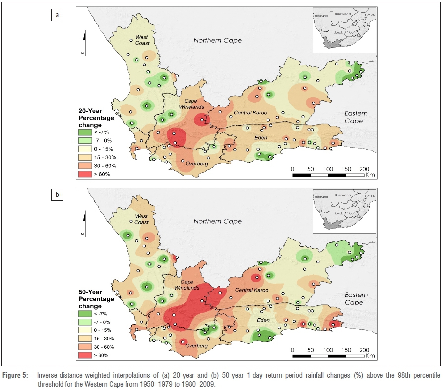
Figure 3 represents the changes in both 20- and 50-year return period rainfall from the initial return level calculated in period 1 (1950-1979) for each individual rainfall station based on the 95th percentile POT data series. A majority of rainfall stations show an increase (>0) in return period rainfalls in the second period (63% for 50-year return period rainfalls), in comparison with the number of rainfall stations that display a decrease (<0) in the magnitude of 50-year storms (37%). We also looked for spatial coherency in the signal by spatially interpolating between stations using ArcGIS (Figures 4 and 5).

The green areas in Figure 4 represent areas of coherent decreases in 20- and 50-year return period rainfalls, while other areas (beige to red) are areas of coherent increases. Two separate regions stand out as areas of coherent decreases: the western mountain escarpment of the West Coast District Municipality (Cederberg to Kouebokkeveld Local Municipalities) and the Central Karoo District Municipality. Most of the remaining parts of the province show increases in the 20- and 50-year rainfalls in the second period, particularly in the mountainous regions of the southern Cape Winelands District Municipality (Drakenstein to Breede Valley local municipalities), and suggest a strong increase in the intensity of extreme return period rainfalls, which potentially enhances their flood risk substantially. There are three pairs of rainfall stations close together in which the pairs show opposing signs of change. Either the data quality of these stations should be questioned, or they are subject to more local-scale influences on rainfall intensity than are the others. Spatial techniques (such as interpolation) are therefore possibly useful for assessing the data quality of these stations by highlighting stations that are different from the general local trend of other nearby gauges.

The results produced using the 98th percentile as the GPD threshold show an expectedly similar pattern to that of the 95th percentile. Increases in 50-year return period rainfall intensity range up to 219% (0022803W Bellevue - between Villiersdorp and Worcester in the Cape Winelands). Using a higher threshold (98th percentile) also increases the proportion of rainfall stations that indicate a rise in the number of 50-year return period rainfalls to 64% - up from 63% using a 95th percentile threshold (Table 2).

Percentile analysis

The use of the GPD method requires a setting of the threshold value to extract the data series. For this study, the 95th and 98th percentiles were accepted as useful estimates of rainfall extremes, as discussed earlier. As the periods 1950-1979 and 1980-2009 need to be viewed as separate data sets for each station, the method entailed calculating separate percentile values for each time period across all rainfall stations. The changes in these percentiles represent changes in the tails of these data distributions, illustrated by the histogram in Figure 6, which represents the percentage of change from the earlier period at the 95th percentile for the given number of stations. The substantial weight of change lies in an increase for the later 1980-2009 period, represented statistically as a positive skewness of 1.32 and the station records are highly skewed to increases in 1-day extreme rainfall. A skewness close to zero should be expected for a comparison in which there is no change between periods.

 

 

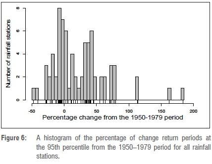
These changes are represented spatially in Figure 7. Here, light areas represent a decrease in 95th percentile between the two periods, while increasingly darker areas represent regions showing 0-10%, 10-20% and >20% increases in the 95th percentile. The Swartland region up the West Coast, as well as a few isolated stations, display a decrease in 95th percentile between the two time periods, while the Kannaland, Oudtshoorn, Laingsburg and Prince Albert Local Municipalities of the Central Karoo and Eden Districts show a marked increase in 95th percentile, which indicates a substantial change in the tails of these distributions. Figure 7 indicates that, in some areas, the threshold value (95th percentile) for the latter period has changed when compared with the original 1950-1979 period. In general, these results show that rainfalls have become more extreme.

 

Conclusions

Our results indicate that the intensity of extreme 1-day rainfalls have shown both increases and decreases across the Western Cape Province in the previous 30 years in comparison to an earlier period. The results are positively skewed towards increases in intensity in the later period across the distribution of the rainfall stations included in this study. The results indicate that the general assumption of stationarity in design rainfall assessments should be strongly questioned. This study provides robust results because the two different methods used provide broadly similar results. These methods can be replicated by future studies in other regions across South Africa and elsewhere and should use the latest rainfall values so as to incorporate more data. The incorporation of additional (more recent) data for the later period to the present in an analysis may change the evaluation further still, as cut-off low weather systems have produced extreme rainfalls in the Western Cape each year from 2010 to 2014 which were not incorporated in this analysis.³

As the magnitude and probabilities of extreme 1-day rainfalls appears to be changing, we also suggest a need for a review of estimation methods and what these mean for design calculations. Our results have implications for the future design and maintenance of infrastructure, as well as water resources management. The statistical methods of evaluating the extreme rainfalls are evolving and it is important that new studies consider these methodological changes. They can add value to the design and decision-making process, and account for changing flood risks, which will benefit society by ultimately reducing deaths, injury and socio-economic losses. Further study is also needed on the changing seasonality of extreme events, which we did not address herein.

We also recommend further investigations into the methods of evaluation, for example including the full rainfall data sequences and using parametric non-stationary approaches by considering changes in the σ and γ parameters of the extreme value distributions with time.²¹ Du Plessis and Burger³⁶ have applied this approach in a limited way to short-duration (<24 h) rainfall intensities for a small number of rainfall stations across South Africa. Such potential future studies would represent analyses of continuous change over time, rather than the comparison of two periods presented here.

 

Acknowledgements

We gratefully acknowledge the South African Weather Service for providing the rainfall data for 2001-2009 for all 76 rainfall stations used in this analysis. We also thank Chané Orsmond for her assistance in data analysis as well as the anonymous reviewers for their valuable insights and recommendations.

 

Authors' contributions

J.H.d.W. wrote significant sections of the paper and undertook the data analysis; he also conceptualised parts of the analysis method. A.C. conceptualised the original approach of using GDP and wrote sections of the paper. J.K. developed the spatial analysis and created the maps.

 

References

1. Katz RW, Brush GS, Parlange MB. Statistics of extremes: Modeling ecological disturbances. Ecology. 2005;86(5):1124-1134. https://doi.org/10.1890/04-0606        [ Links ]

2. Holloway A, Fortune G, Chasi V. RADAR Western Cape review: Risk and development annual review. Cape Town: PeriPeri Publications; 2010.         [ Links ]

3. Pharoah R, Holloway A, Fortune G, Chapman A, Schaber E, Zweig P. Off the RADAR: Synthesis report. High impact weather events in the Western Cape, South Africa 2003-2014. Stellenbosch: Research Alliance for Disaster and Risk Reduction, Department of Geography and Environmental Studies; 2016.         [ Links ]

4. Field CB, Barros V, Stocker TF, Qin D, Dokken DJ, Ebi KL, et al., editors. Managing the risks of extreme events and disasters to advance climate change adaptation. A special report of Working Groups I and II of the Intergovernmental Panel on Climate Change. Cambridge: Cambridge University Press; 2012. https://doi.org/10.1017/CBO9781139177245        [ Links ]

5. SANRAL. Drainage manual. 5th ed. Pretoria: SANRAL; 2007.         [ Links ]

6. Milly P, Betancourt J, Falkenmark M, Hirsch R, Kundzewicz Z, Lettenmaier D, et al. Stationarity is dead: Whither water management? Science. 2008;319:573-574. https://doi.org/10.1126/science.1151915        [ Links ]

7. Milly PCD, Wetherald RT, Dunne KA, Delworth TL. Increasing risk of great floods in a changing climate. Nature. 2002;415:514-517. https://doi.org/10.1038/415514a        [ Links ]

8. Trenberth KE, Dai A, Rasmussen RM, Parsons DB. The changing character of precipitation. Bull Am Meteorol Soc. 2003;84:1205-1217. https://doi.org/10.1175/BAMS-84-9-1205        [ Links ]

9. Bates BC, Kundzewicz ZW, Wu S, Palutikof JP, editors. Climate change and water. Technical Paper of the Intergovernmental Panel on Climate Change. Geneva: IPCC Secretariat; 2008.         [ Links ]

10. Mason S, Waylen P, Mimmack G, Rajaratnam B, Harrison J. Changes in extreme rainfall events in South Africa. Clim Change. 1999;41:249-257. https://doi.org/10.1023/A:1005450924499        [ Links ]

11. Easterling D, Evans J, Groisman P, Karl T, Kunkel K, Ambenje P. Observed variability and trends in extreme climate events: A brief review. Bull Am Meteorol Soc. 2000;81:417-425. https://doi.org/10.1175/1520-0477(2000)081<0417:OVATIE>2.3.CO;2        [ Links ]

12. Richard Y, Fauchereau N, Poccard I, Rouault M, Trzaska S. 20th century droughts in Southern Africa - Spatial and temporal variability, teleconnections with oceanic and atmospheric conditions. Int J Climatol. 2001;21:873-895. https://doi.org/10.1002/joc.656        [ Links ]

13. Groisman P, Knight R, Easterling D, Karl T, Hegerl G, Razuvaev V. Trends in intense precipitation in the climate record. J Climate. 2005;18:1326-1350. https://doi.org/10.1175/JCLI3339.1        [ Links ]

14. Kruger AC. Observed trends in daily precipitation indices in South Africa: 1910-2004. Int J Climatol. 2006;26:2275-2285. https://doi.org/10.1002/joc.1368        [ Links ]

15. New M, Hewitson B, Stephenson DB, Tsiga A, Kruger A, Manhique A, et al. Evidence of trends in daily climate extremes over southern and west Africa. J Geophys Res. 2006;111, Art. #D14102, 11 pages. https://doi.org/10.1029/2005JD006289        [ Links ]

16. Katz RW. Statistics of extremes in climate change. Clim Change. 2010;100:71-76. https://doi.org/10.1007/s10584-010-9834-5        [ Links ]

17. Alexander W. Flood hydrology for Southern Africa. Pretoria: Southern African Committee for Large Dams; 1990.         [ Links ]

18. Smithers JC, Schulze RE. Design rainfall and flood estimation in South Africa. Water Research Commission project no: K5/1060. Pretoria: Water Research Commission; 2002. Available from: http://www.wrc.org.za/Knowledge%20Hub%20Documents/Research%20Reports/1060%20web.pdf        [ Links ]

19. Langbein WB. Annual floods and the partial-duration flood series. Trans Am Geophys Union. 1949;30(60):879-891.         [ Links ]

20. UCAR. Statistics of weather and climate extremes [database on the Internet]. No date [cited 2016 Sep 02].         [ Links ] Available from: https://www.isse.ucar.edu/extremevalues/extreme.html

21. Coles S. An introduction to statistical modelling of extreme values. London: Springer; 2001. https://doi.org/10.1007/978-1-4471-3675-0_3        [ Links ]

22. R Core Team. R: A language and environment for statistical computing [homepage on the Internet].         [ Links ] No date [cited 2016 Sep 03]. Available from: http://www.R-project.org/

23. Katz R, Parlange M, Naveau P. Statistics of extremes in hydrology. Adv Water Resour. 2002;25:1287-1304. https://doi.org/10.1016/S0309-1708(02)00056-8        [ Links ]

24. Gilleland E, Katz RW. Analysing seasonal to interannual extreme weather and climate variability with the Extremes Toolkit [document on the Internet]. c2006 [cited 2016 Sep 03].         [ Links ] Available from: http://www.isse.ucar.edu/extremevalues/Gilleland2006.pdf

25. Papalexiou SM, Koutsoyiannis D, Makropoulos C. How extreme is extreme? An assessment of daily rainfall distribution tails. Hydrol Earth Syst Sci. 2013;17:851-862. https://doi.org/10.5194/hess-17-851-2013        [ Links ]

26. Scarrott C, MacDonald A. A review of extreme value threshold estimation and uncertainty quantification. REVSTAT Stat J. 2012;10(1):33-60. Available from: http://www.ine.pt/revstat/pdf/rs120102.pdf        [ Links ]

27. Stephenson A. Package 'ismev' [homepage on the Internet].         [ Links ] c2016 [cited 2016 Sep 16]. Available from: https://cran.r-project.org/web/packages/ismev/index.html

28. Moberg A, Jones PD, Lister D, Walther A, Brunet M, Jacobeit J, et al. Indices for daily temperature and precipitation extremes in Europe analyzed for the period 1901-2000. J Geophys Res. 2006;111, Art. #D22106, 25 pages. https://doi.org/10.1029/2006JD007103        [ Links ]

29. Eagleson PS. Some limiting forms of the Poisson distribution of annual station precipitation. Water Resour Res. 1981;17(3):752-757. https://doi.org/10.1029/WR017i003p00752        [ Links ]

30. Lynch SD. Development of a raster database of annual, monthly and daily rainfall for Southern Africa. Water Research Commission report no. 1156/1/03 [document on the Internet].         [ Links ] c2004 [cited 2016 Sep 02]. Available from: http://www.wrc.org.za/knowledge%20hub%20documents/research%20reports/1156-1-04.pdf

31. Li Y, Cai W, Campbell E. Statistical modeling of extreme rainfall in southwest Western Australia. J Clim. 2005;18:852-863. https://doi.org/10.1175/JCLI-3296.1        [ Links ]

32. Neville SE, Palmer MJ, Wand MP. Generalised extreme value additive model analysis via mean field variational Bayes. Aust N Z J Stat. 2011;53(3):305-330. https://doi.org/10.1111/j.1467-842X.2011.00637.x        [ Links ]

33. Zang X, Hegerl G, Zwiers FW, Kenyon J. Avoiding inhomogeneity in percentile-based indices of temperature extremes. J Clim. 2005;18:1641-1651. https://doi.org/10.1175/JCLI3366.1        [ Links ]

34. Klein Tank A, Zwiers F, Zhang X. Guidelines on analysis of extremes in a changing climate in support of informed decisions for adaptation: Technical report, climate data and monitoring. Report number WCDMP-no. 72. Geneva: World Meteorological Organization; 2009.         [ Links ]

35. Kovacs ZP, Du Plessis DB, Bracher PR, Dunn P, Mallory GCL. Documentation of the 1984 Domoina floods. Technical report no. 122 for the Department of Water Affairs [document on the Internet].         [ Links ] c1985 [cited 2016 Sep 02]. Available from: https://www.dwa.gov.za/iwqs/reports/tr/TR_122_1984_Domoina_floods.pdf

36. Du Plessis J, Burger G. Investigation into increasing short-duration rainfall intensities in South Africa. Water SA. 2015;14(3):416-424. https://doi.org/10.4314/wsa.v41i3.14        [ Links ]

 

 

Correspondence:
Jan de Waal
Email: janniedw@sun.ac.za

Received: 14 Aug. 2016
Revised: 20 Dec. 2016
Accepted: 15 Feb. 2017

 

 

FUNDING None