RESEARCH ARTICLE

 

Changing boundaries: Overcoming modifiable areal unit problems related to unemployment data in South Africa

 

 

Gina Weir-Smith^{I, II}

^IResearch Data Management Centre, Human Sciences Research Council, Pretoria, South Africa
^IIHonorary Research Fellow, School of Geography, Archaeology & Environmental Studies, University of the Witwatersrand, Johannesburg, South Africa

Correspondence

 

 

---

ABSTRACT

The longitudinal comparison of census data in spatial format is often problematic because of changes in administrative boundaries. Such shifting boundaries are referred to as the modifiable areal unit problem (MAUP). This article utilises unemployment data between 1991 and 2007 in South Africa to illustrate the challenge and proposes ways to overcome it. Various censuses in South Africa use different reporting geographies. Unemployment data for magisterial districts of census 1991 and 1996 were re-modelled to the 2005 municipal boundaries. This article showed that areal interpolation to a common administrative boundary could overcome these reporting obstacles. The results confirmed more accurate interpolations in rural areas with standard errors below 3300. Conversely, the largest errors were recorded in the metropolitan areas. Huge increases in unemployment between 1996 and 2001 statistics were also evident, especially in the metropolitan areas. Although such areas are more complex in nature, making it more difficult to accurately calculate census data, the increase in unemployment could also be the result of census taking methods. The article concludes that socio-economic data should be available at the smallest possible geographic area to ensure more accurate results in interpolation. It also recommends that new output areas be conceptualised to create a seamless database of census data from 1991 to 2011 in South Africa.

Keywords: data aggregation; unemployment; areal interpolation; socio-economic trends; census

---

 

 

Introduction

One of the main interests of census and population researchers is the study of socio-economic change.¹ The study of change is especially important to answer questions at a local scale, for example, a suburb or municipality. However, such comparisons over time are difficult because census collection methods and definitions as well as reporting geographies change.

This article seeks to find a solution to the problem of shifting boundaries as exemplified in the case of unemployment trends over time in South Africa. The problem of shifting boundaries is referred to as the modifiable areal unit problem (MAUP). Currently there is limited literature available on overcoming the MAUP in South Africa using socio-economic data. Although there are some attempts to build historical Geographic Information System socio-economic data sets in South Africa, their methodologies are not yet documented in the literature.²

To minimise the effects of the MAUP administrative units should be as disaggregated as possible.³ The MAUP is composed of two problems: firstly, the scale problem, where different results can occur when one set of areal units is aggregated into a fewer number of larger units for analysis; and secondly, the aggregation problem, where different results can be obtained when boundaries of spatial entities are arranged in different ways. In this article, the MAUP specifically refers to the change in geographical units of analysis.

Given the challenge of enumeration area (EA) and magisterial district boundary changes in South Africa since 1991, this article seeks to find a methodological solution for overcoming modifiable areal unit problems in South African census data. Unemployment, which is extremely high in South Africa, and often used as an indication of socio-economic well-being, is used here to illustrate the challenge of the MAUP

Challenges in integrating spatial and temporal data over time

The historical linking of data in Geographic Information Systems (GIS) faces two major problems. Firstly, available commercial software is ill suited to temporal GIS. Secondly, and partly in consequence, historical GIS construction is very expensive, especially because of labour costs related to extensively solving challenges.⁴ These factors influence any longitudinal spatial analysis of socio-economic conditions in South Africa.

Census data are the only data at a national level that include all citizens and cover the full geographical extent of the country. Therefore these data were accepted as the spatially most comprehensive data on unemployment in South Africa. There are, however, arguments that the census is not as accurate as the Labour Force Survey (LFS) and Quarterly Labour Force Survey (QLFS) in measuring unemployment because it does not ask questions about the reasons for not being employed. Nevertheless, it was important to use the census, which provides the most spatially detailed data in order to build a national understanding of an issue at a spatially disaggregated (sub-provincial) level.

The study of change over time through reference to census data is fraught with difficulties because of operational changes made between censuses to improve their relevance and reliability, and because of differences in the degree to which they achieved their aims.⁵ Although aggregation to geographical areas is a near-universal feature of census information, it is fundamentally difficult to accommodate.⁶ Data created by interpolation are estimates that will inevitably contain a certain degree of error.⁷ The accuracy of areal interpolation, moreover, will vary according to the nature of the variable being interpolated, the nature of the ancillary data and the shape and size of both the source and target units.⁷

Further challenges in terms of integrating spatial data over time are the scale of administrative units for analysis and the linking of the attribute data from various years to the spatial data.^8,9 Although these two aspects are related, they pose distinct ways of dealing with the problem. The remainder of this section deals with these two issues separately using unemployment data to illustrate them.

Means of addressing the modifiable areal unit problems Spatial solutions

One of the ways to link different census geographies is through areal interpolation. Areal interpolation was used to create a temporal census database for Europe and areal weighting specifically was used to achieve this.⁴ Areal weighting is based on the assumption that data are distributed homogeneously across each source unit. Count data for a variable y are interpolated from the source zones to the target zones using the formula:

yt = Σ[Ast / As χ ys] Equation 1

where yt is the estimated value for the target zone, ys is value for the source zone, As is the area of the source zone, and Ast is the area of the zone of intersection between the source and target zones.¹⁰ The assumption of a homogeneous population distribution is, however, unrealistic for most socio-economic applications. Although a number of studies have tried to render this mathematical model more flexible by introducing ancillary data to the model, no matter how good the technique, areal interpolation will inevitably contain some error, the impact of which will vary from polygon to polygon.⁵

The nature of the data being interpolated also determines the accuracy of the results.¹¹ Some attempts have been made to calculate the interpolation error, but most of these are limited because they show global goodness of fit and do not provide detail at the level of individual data values. In statistical terms 'goodness of fit' refers to the confidence with which a model can be presented while 'global' indicates the fit of that model at the general level. Poorer results are obtained as the scale of the output area is reduced and more accurate interpolation is achieved in rural areas.¹² Urban areas are complex and there seems to be no easy solution to the challenge. The choice of an interpolation strategy has a strong influence on model results, and thus on potentially far-reaching policy decisions.¹³ It is therefore important to use the correct methodology.

Three types of re-aggregation criteria are offered to create new areal units from census data: firstly, areas that possess similar levels of heterogeneity for the specific variable of interest; secondly, areas that are of an approximately equal size and shape; and thirdly, areas that provide an efficient partitioning of space and are of similar nature.¹⁴

Besides areal interpolation, small area grids and automated zoning can be used. These methods are briefly discussed and some examples given. The centroids of the1991 enumeration districts in England, Wales and Scotland were used in an areal aggregation solution to aggregate data to the 1981 wards.¹ The same was done for the 1971 enumeration district data, whereafter it was aggregated to higher geographies. A controlled public access system was created, which delivers a number of user defined outputs.

In a different technique, root mean square (RMS) error is used to quantify the error introduced in simulations. This is based on the average differences between the estimated values of the variable and its known actual values.¹⁵

Another solution to represent data from small areas in a re-aggregated format is the use of grids. Small area grids should be more than 1 km (5 km is desired).¹⁶ On the other hand, small grids have the risk of containing below-threshold numbers of people thereby compromising anonymity. A greater understanding of the uses to which grid-based geographies are put is required in order to assess whether such grids would prove useful.¹⁶ Research showed that polygon methods have a lower map accuracy error than their grid-based counterparts, though the difference was not statistically significant.¹⁷

The most appropriate response to the MAUP is to design purpose-specific zonal systems.³ A study using such methods aggregated data from the household level to small areas (data zones) using the Community Survey (CS) 2007 data in South Africa.¹⁸ The authors used multi-level modelling to calculate a 'best linear unbiased estimator' of multiple deprivation for each data zone in the country. The data zones were calculated based on a data zone code provided by Statistics South Africa (Stats SA) and multi-level modelling was used for attribute data.

Continual boundary revision of census areas in order to retain a degree of equality of population sizes renders the separation of population change from boundary change particularly difficult.¹⁹ It would therefore become difficult to detect real population change, because such change would always be associated with a change in boundaries.

Temporal solutions

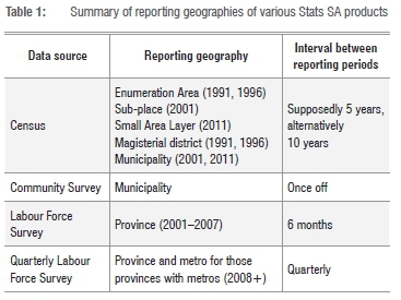
Stats SA produces all the official data sets for South Africa. These include censuses, LFS and CS, among others. Censuses take place every 5-10 years and cover the total population, while the QLFS takes place quarterly and relies on a national sample of about 30 000 households.²⁰ The QLFS reports unemployment figures at a provincial level and distinguishes between metropolitan and non-metropolitan areas within a province, while censuses report unemployment data at an EA, magisterial district or municipality level. In the absence of a census in 2006, a CS was conducted in 2007 and reported data at a municipal level.

Table 1 summarises the reporting geographies of Stats SA products and shows that it varies significantly between different products. Census, which contains the most detailed spatial data, takes place every 5 years or alternatively every 10 years. Labour Force Surveys only report unemployment at a provincial level, i.e. one record for every province.

 

 

Stats SA has admitted that the following factors complicate the use of comparative studies that rely on data collected in South African censuses.²¹ Firstly, the continuous and complete changing of administrative boundaries; secondly, the revision of the set of EAs that was used in Census 1996; and thirdly, the decision not to release the Census 2001 data at EA level. The fact that spatial units from the various censuses and surveys are not the same at different periods creates problems for researchers attempting to establish a seamless, temporal database for analysis of unemployment.

The effect of census change in South Africa

EAs are essentially used to make the work of the census enumerator manageable, so these boundaries change between censuses. The number of EAs has increased significantly since 1991 to accommodate changes in population growth, urbanisation and so forth. Most provinces had a moderate decline in the number of EAs between 1996 and 2001 while the total number of EAs in the 2011 census increased to around 104 000.²²

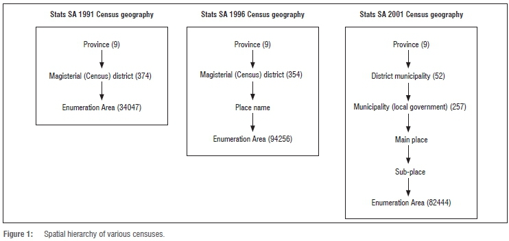
Figure 1 illustrates the differences between the spatial units in the various censuses. In 1991, census data were gathered at an EA level and disseminated at a magisterial district level. In 1996, the situation was the same except that data were released at an EA level as well. In 2001, Stats SA created the first official census geography with a number of spatial levels; and although the data were collected at an EA level, the information was only released at a sub-place level.

In order to obtain a trustworthy understanding of spatial changes in unemployment patterns over a given time span, data from four different periods are required. Data from only three periods might possibly not show a trustworthy trend in unemployment. The most recent censuses in South Africa were conducted in 2011, 2001, 1996, 1991, 1985, 1980 and 1970.

The censuses of 1985 and 1980 did not include all South Africans and were therefore problematic for this research. Although the census of 1970 included South Africans of all race groups, labour patterns have changed significantly since then and would not be relevant to current, post-apartheid South Africa. Therefore, another data source was considered, the CS 2007, which was a large sample survey that presented results at the level of the local municipal boundaries of 2005.²³

 

Methodology

The challenge of analysing unemployment spatially over time is the incompatibility of various spatial units of data representation. Ideally, areal interpolation should be done at the most detailed level spatially and in the case of South Africa, this would be the EA level. As the EA is the smallest geographical unit, it should make aggregation to higher-level geographical units easy and achievable. However, the difficulty in matching attribute and spatial data (1996 census) and the lack of attribute data (1991 census) makes this difficult to attain.

For this research, the linking of different census geographies was achieved by using areal interpolation to transfer data from one set of boundaries to another. The 2005 municipality boundaries were used as the common denominator - part of a spatial hierarchy developed by Stats SA for the 2001 census. This hierarchy started with the EA as the lowest building block, then sub-place, main place, local municipality and province (see Figure 1). The municipal boundaries for 2005 were chosen as the preferred target area, because they represented a recent administrative division useful for displaying temporal change and they were easily linked to the 2001 and 2007 data.

Other methodologies that could have been considered were, for example, disaggregation based on dasymetric mapping but this method required additional verification through ancillary data.^2,17,24 The lack of an additional data set related to economic activities at municipal level would makes the validation process difficult.²⁵

Data sources

Census data constitute the only data source at a national level that aims to include all citizens and all geographical areas. It was therefore accepted that the census was the most comprehensive spatial data set on unemployment in the country. Census and CS data were obtained from Stats SA and the Human Sciences Research Council (HSRC) of South Africa.

In the 1991 census, unemployment statistics data were not directly calculated; these figures were generated by subtracting the number of employed people from the economically active population. The estimated undercount in 1991 was an average of 12.7% across all race groups.²⁶ Stats SA provided the number of unemployed people per magisterial district in the 1996 census. The statistics for these two censuses were therefore in comparable formats. The estimated undercount in 1996 was 10.7%.²⁷

The 2001 census attribute data were not released at an EA level for reasons of confidentiality²¹ but were made available at a sub-place level and could therefore be aggregated to municipal level. The estimated undercount for people in the 2001 census was 17.6%.²⁸ CS 2007 released data on the number of unemployed people as well as the economically active population at municipal level. The level of analysis was therefore standardised to municipalities and depended on a certain measure of areal interpolation - the most optimal way of standardising the unit of analysis.⁸

It was decided that the CS 2007 rather than the 1970 Census would be used because the CS was closer in time to the other censuses used. Although the CS 2007 was a survey, the sample size of 949 105 persons was large enough to enable reporting of the findings at municipal level.

The correction of the undercount in census 1996 and census 2001 was undertaken during the post-enumeration survey. After the 1991 census, an adjustment for the undercount was made and the corrected statistics were released. In the CS 2007, the estimation process was based on the ratio method of projecting geographic subdivisions to determine the populations of district councils and municipalities. This article did not investigate the undercount corrections per se, and assumed that the data released by Stats SA were accurate and thus constituted the most complete data available spatially.

Aggregating data

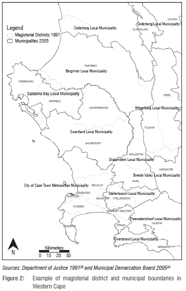
Areal aggregation is usually from a source polygon layer to a target polygon layer. Figure 2 shows a layout of the magisterial and municipal boundaries in Western Cape and displays that magisterial districts were largely within the boundaries of metropolitan areas. In non-metropolitan municipalities, magisterial boundaries sometimes extended beyond those of the municipality. Magisterial districts were used as the source polygon and municipalities as the target polygon.

 

 

A geostatistical process of areal-based interpolation was followed and it initially created a prediction surface from the source polygons. Predictions and standard errors were calculated for all points within and between the input polygons (magisterial districts). As unemployment statistics are continuous, the input was defined as Gaussian polygonal because the polygons of collection were fairly large.³¹ A standard error of the predicted unemployment value was calculated for each polygon and is further discussed in conjuction with Figure 5.

During the second part of the interpolation, a process of cross-validation and validation was followed to make a decision as to which model provided the best predictions. These predictions, along with standard errors, were calculated for each municipal polygon. Some of the other components of this variogram stage included model type, lag size and lattice spacing (Figure 3). The variogram model can either be circular, spherical, exponential, tetraspherical, pentaspherical, Gaussian, K-Bessel, Stable and J-Bessel. The spherical model is the most widely used variogram model and assumes that covariance reaches a value of zero at a specific distance.³² K-Bessel and Stable models produce the best results because they take an additional shape parameter that allows the model to change curvature.³³ However, they also take the longest to process.

 

 

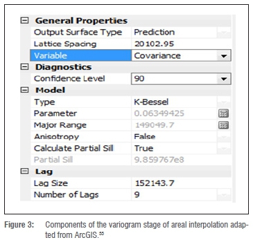
Lag size refers to the number of adjacent cells in a straight horizontal or straight vertical line from the centre to the edge of the figure and usually the lag size multiplied by the number of lags should be less than one-half of the largest distances in one's data set.³¹ Fewer lags usually improve the covariance value. Lattice spacing refers to the number of points used within each polygon to build the semi-variogram and the smaller the spacing, the longer it takes to generate the semi-variogram and the more memory is consumed.

For a model to provide accurate predictions, the standardised mean error should be close to 0, the root-mean-square error and average standard error should be as small as possible and the root-mean square standardised error should be close to 1.³¹

1991 and 1996 Census

For the 1991 data, a spherical model was used and twelve lags were performed within a confidence level of 90%. The final model of the 1996 data used a K-Bessel model with nine lags, a lag size of 100 000 and a lattice spacing of 18 000. The K-Bessel model is more stable, but also takes longer to process. If the models were correctly specified, one would expect 90% of the empirical co-variances to fall within the confidence intervals.

2001 Census

To obtain unemployment figures for 2001, data were downloaded from the 'Statistics Sa Interactive data' website (http://interactive.statssa.gov.za:8282/webview/). Because these data were pre-customised for the 2005 municipal boundaries, there was no need to perform any calculations on the data to re-align them with the 2005 boundaries.

2007 Community survey

The 2007 CS data were downloaded from the 'Statistics SA Interactive data' website. The data reported results at the spatial level of the 2005 municipal boundaries. The unemployment rate was then calculated using the following formula (which excluded institutions like hostels, retirement homes, etc. and 'unspecified' responses):

[unemployed/(employed + unemployed)] χ 100 Equation 2

Data for each year being analysed had to be treated individually because there was no global solution to the spatial problems encountered. The unemployment definitions remained the same and were therefore comparable. Data pre-processing was time-consuming, which confirmed the assertion that temporal construction in GIS is a costly exercise.³⁴ In this case the data were obtained free of charge, but it took a considerable amount of time to process the data to a comparable format.

 

Findings and discussion

Results from the 1991 areal interpolation show that 8 of the 13 points were within the 90% confidence level so the model is therefore acceptable. Furthermore, the root mean squared standardised error was 1.2, therefore the predicted standard errors were valid because they are close to 1.

Figure 4 displays the variogram with averaged values (thick crosses) for the 1996 data and more than 90% of the empirical co-variances fell within the confidence intervals (long bars). The model was therefore acceptable. The mean squared standardised error was 0.9 and therefore the predicted standard errors were valid.

Figure 5 displays the standard errors for the 1996 data in a quantile map for the target layer, namely the 2005 municipalities. The largest errors were recorded in metropolitan areas like Cape Town, Johannesburg, Pretoria, Ekurhuleni and eThekwini. However, the large errors were not restricted to metropolitan municipalities and also appeared in other urban municipalities for example along the coast of KwaZulu-Natal, around Polokwane in Limpopo, the southern coast and selected municipalities in the Western Cape. This finding strengthens literature trends that established more accurate interpolation results in rural areas.

Table 2 indicates that in 1991, 5 of the 257 municipalities had more than 1000 EAs. All these municipalities were metropolitan areas. In 1996, 11 of the 257 municipalities (4.2%) had more than 1000 EAs. Besides the metropolitan areas, a number of municipalities in the Eastern Cape (including the former Transkei) and in Gauteng and KwaZulu-Natal had more than 1000 EAs each.

The implication is that in 1996 in 4.2% of municipalities, the aggregation error could be bigger than the census undercount. For the 1991 data, this would be 2% of municipalities. Therefore, these simple aggregation techniques would result in an aggregation error in a small percentage of the data which could be considered acceptable.¹

Results from the areal interpolation of the 1991 and 1996 magisterial districts used in this article yielded the statistics shown in Table 3. Selected municipalities are reflected in the table as there are too many municipalities to portray at once. The table shows results for two municipalities in each of the nine provinces, representing different types of entities - urban/metropolitan and rural. The data in the table are sorted alphabetically by province.

The municipality discussed here with the highest unemployment rate was Nongoma, in KwaZulu-Natal. This municipality showed continuous high levels of unemployment in 1996, 2001 and 2007. There was an increase of about 20% in unemployment between 1996 and 2001, while the figures declined somewhat in 2007.

Large increases were seen between the two sets of 1996 and 2001 statistics, especially in the metros, for example, the City of Cape Town that recorded 6.9% unemployment in 1996. In metros like Cape Town, Johannesburg and eThekwini, the same differences prevailed in 2001 and 2007. The inflated unemployment rates for 2001 can be ascribed to misclassification, where employment status shifted some of discouraged job seekers to outside the economically active band.²⁵

Sparsely populated areas like Matatiele (Eastern Cape) and Kamiesberg (Northern Cape) also showed stark differences in the percentages of unemployed people. The official statistics (that is, those sourced from Stats SA) show peak unemployment figures in 2001 with moderate declines in 2007.

Considering the different ways of overcoming the census MAUP in South Africa, the ideal solution would be to use the boundaries of existing small area features like EAs or sub-places. The challenge of not having attribute data for all EAs in 1991 and 1996 made this difficult to attain. The same shortcoming would apply to small area grids and automated zoning, because the lack of underlying data would make it difficult to achieve results at small area levels. Automated zoning could be used at higher level geographies like municipalities, but as data existed for magisterial districts in 1991 and 1996, it was more opportune to aggregate these to the 2005 municipalities.

A limitation of the uncertainty estimates provided by areal interpolation methods is that they are likely to underestimate the real uncertainty of the associated spatial predictions. This is based on the fact that these methods are two-stage processes, where a variogram model is estimated in the first stage and prediction and uncertainty equations are applied in the second stage. The second stage equations treat the first stage variogram model as true and known.³⁷ To address this, the documentation of any spatial interpolation exercise can explicitly recognise their bias toward underestimating uncertainty. Decision makers and other users of the modelling results can then decide for themselves how best to adjust their interpretation based on this information.³⁷

Kriging-based methods such as areal interpolation are by definition smoothing operators. Although the formulas are true to the data, the relatively smooth spatial interpolation surface they provide may not capture all the underlying variation of the process they are attempting to describe.³⁷ In this research a discreet input and output value was calculated for unemployment in a specific municipality. The value cannot be reflective of all unemployment rates across that municipality, e.g. unemployment rates in a township is not the same as unemployment in a suburb or the city centre. In fact, to require an interpolation model to be highly accurate at each specific location is an unfair expectation, because it is supposed to provide a spatial description of the unemployment situation in general.³⁷

 

Conclusion and recommendations

Empirical analysis of past trends is vital for extending knowledge of the processes producing change. This article aimed to create a spatially comparable unemployment data set from 1991 to 2007. Although there are enormous challenges related to constructing a time-continuous GIS data set, many of these were overcome by aggregating data from magisterial district boundaries to municipalities. The research has created a spatio-temporal data set which could be used as a basis for future research and can be regarded as work in progress.

Accuracy was reflected in prediction errors for each polygon and this lends validity to the findings. The predicted standard errors for the 1996 data were valid, because the mean squared standardised error was 0.9 which is close to the acceptable value of 1. Similarly, the 1991 results were acceptable because the root mean standardised error was close to 1.

Inaccuracies in the 1991 and 1996 EA level data made it difficult to accurately aggregate to higher geographical entities. The compromise was to aggregate data from magisterial districts for these years to municipal boundaries. Future research on the South African data could include calculations such as weighting the interpolation process, which might increase the confidence with which one could report reasonable results. Weighting could be done using population density or road density. However, if unemployment statistics are released at a local scale such as sub-place, weighting would not be necessary, because the variance within a polygon should be minimal.

The areal interpolation results indicated that the largest errors were recorded in metropolitan areas and other urban municipalities. This finding supports literature trends which established that more accurate interpolation tends to be in rural areas. Further research could investigate the possibility of using small grids as an alternative method to aggregate unemployment data and compare results with the findings of this research.

The best way to overcome some of the errors in the findings is to ground-truth the data. This would include physically counting how many people were unemployed in a specific area. As the data date from 1991 and 1996, the only proxy for such a count would be to use satellite imagery of that time, count the number of dwellings and then estimate the number of unemployed based on a ratio of employed people vs unemployed people. To ground-truth data in the field is a very costly exercise and that is one of the reasons why a census is not conducted every year.

A lack of spatially detailed data is at the helm of this research problem and other methods like dasymetric mapping, which is dependent on supplementary data at a detailed spatial level, will suffer the same shortcomings. It is recommended that aggregated data on unemployment and other socio-economic variables be created from the smallest spatial unit, that is, EA or sub-place. However, in the South African case, EA boundaries changed again with Census 2011, which means that researchers would have to once again recalculate socio-economic data to fit the new features.

A further possible solution could be to impute unemployment data for 1991 and 1996 EAs in cases where such data are missing. This would allow the aggregation of unemployment and other census data to larger geographical units. Data incompatibilities could also be overcome by creating new output areas that would be able to serve as target areas for areal interpolation from the 1991 census onwards. Alternatively, Census 2011 EA centroids could be used to interpolate attribute data from EAs of earlier years.

By highlighting and addressing some of the spatial and attribute data challenges of publicly available unemployment data in South Africa, this article has created a base for future research using the same data sources. The research aimed to create a comparative geographical database where socio-economic change is not the result of boundary changes. This article has shown that there are still a number of hurdles to overcome in creating a seamless database of census data since 1991. Hopefully the results from Census 2011 will allow the creation of a longitudinal data set of spatial socio-economic trends in South Africa at a detailed geographical level.

 

Acknowledgements

The author would like to thank Adlai Davids and Fethi Ahmed for valuable input received on earlier versions of this article.

 

References

1. Martin D, Dorling D, Mitchell R. Linking censuses through time: Problems and solutions. Area. 2002;34:82-91. http://dx.doi.org/10.1111/1475-4762.00059        [ Links ]

2. Mans G. Developing a geo-data frame using dasymetric mapping principles to facilitate data integration [document on the Internet]. c2010 [cited 2012 April 06]. Available from: http://www.gap.csir.co.za/gap/gap-applications        [ Links ]

3. Openshaw S. The modifiable area unit problem. Concepts and techniques in modern geography 38. Norwich: Geo Books; 1984.         [ Links ]

4. Gregory IN, Southall H. Spatial frameworks for historical censuses: The Great Britain historical GIS. In: Hall PK, McCaa, R, Thorvaldsen G, editors. Handbook of historical microdata for population research. Minneapolis: Minnesota Population Center; 2000. p. 319-33.         [ Links ]

5. Champion AG. Analysis of change through time. In: Openshaw S, editor. Census users' handbook. Cambridge: GeoInformation International; 1995. p. 307-335.         [ Links ]

6. Martin D. 2000. Census 2001: Making the best of zonal geographies. Paper delivered at The Census of Population: 2000 and Beyond; 2001 June 23; Manchester, England.         [ Links ]

7. Gregory IN, Ell PS. Error-sensitive historical GIS: Identifying areal interpolation errors in time-series data. Int J Geogr Inf Sci. 2006;20(2):135-152. http://dx.doi.org/10.1080/13658810500399589        [ Links ]

8. Gregory IN, Marti-Henneberg J, Tapiador F. A GIS reconstruction of the population of Europe, 1870 to 2000 [document on the Internet]. c2008 [cited 2011 Jul 19]. Available from: http://web.udl.es/dept/geosoc/europa/cas/img/GIS%20Approaches%20-%20resubmission.6.06.pdf        [ Links ]

9. Martin D, Gascoigne R. Change and change again: Geographical implications for intercensal analysis. Area. 1994;26:133-141.         [ Links ]

10. Goodchild MF, Lam NSN. Areal interpolation: A variant of the traditional problem. Geo-Processing. 1980;1:297-312.         [ Links ]

11. Gregory IN. The accuracy of areal interpolation techniques: Standardising 19th and 20th century census data to allow long-term comparisons. Comput Environ Urban. 2002;26:293-314. http://dx.doi.org/10.1016/s0198-9715(01)00013-8        [ Links ]

12. Martin D. Extending the automated zoning procedure to reconcile incompatible zoning systems. Int J Geogr Inf Sci. 2003;17:181-196. http://dx.doi.org/10.1080/713811750        [ Links ]

13. Goodchild MF, Anselin L, Deichmann U. A framework for the areal interpolation of socioeconomic data. Environ Plan. 1993;25:383-397. http://dx.doi.org/10.1068/a250383        [ Links ]

14. Charlton M, Rao L, Carver S. GIS and the census. In: Openshaw S, editor. Census users' handbook. Cambridge: GeoInformation International; 1995. p. 133-166. http://dx.doi.org/10.1068/a270425        [ Links ]

15. Fisher PF, Langford M. Modelling the errors in areal interpolation between zonal systems by Monte Carlo simulation. Environ Plan. 1995;27:211-224. http://dx.doi.org/10.1068/a270211        [ Links ]

16. Duke-Williams O, Rees P. Can census offices publish statistics for more than one small area geography? An analysis of the differencing problem in statistical disclosure. Int J Geogr Inf Sci. 1998;12:579-605. http://dx.doi.org/10.1080/136588198241680        [ Links ]

17. Eicher CL, Brewer CA. Dasymetric mapping and areal interpolation: Implementation and evaluation. Cartogr Geogr Inf Sci. 2001;28:125-138. http://dx.doi.org/10.1559/152304001782173727        [ Links ]

18. Noble M, Dibben C, Wright G. The South African index of multiple deprivation 2007 at datazone level (modelled). Pretoria: Department of Social Development; 2010.         [ Links ]

19. Geddes A, Flowerdew R. Geographical considerations in designing policy-relevant regions. Proceedings of the 3rd AGILE Conference on Geographic Information Science; 2000 May 25-27; Helsinki: Finland. p. 80-81        [ Links ]

20. Statistics South Africa (Stats SA). Guide to the Quarterly Labour Force Survey August 2008. Pretoria: Stats SA; 2011.         [ Links ]

21. Statistics South Africa. Using the 2001 Census: Approaches to analysing data [document on the Internet]. c2007 [cited 2010 Aug 22]. Available from: http://www.statssa.gov.za/Publications/CensusHandBook/CensusHandbook.pdf        [ Links ]

22. Statistics South Africa (Stats SA). Census 2011: EA spatial data. Data set: Pretoria: Stats SA; 2012.         [ Links ]

23. Statistics South Africa (Stats SA). General Household Survey: Report no. P0318. Pretoria: Stats SA; 2008.         [ Links ]

24. Mennis J. Generating surface models of population using dasymetric mapping. Prof Geogr. 2003;55(1):31-42.         [ Links ]

25. Hakizimana JV. Small area estimation of unemployment for South African labour market statistics [Msc dissertation]. Johannesburg: University of Witwatersrand; 2011.         [ Links ]

26. Statistics South Africa. Census 1991: Explanatory notes [document on the Internet]. no date [cited 2011 Apr 15]. Available from: http://interactive.statssa.gov.za:8282/metadata/censuses/1991/RSA/RSA1991.htm        [ Links ]

27. Statistics South Africa (Stats SA). Calculating the undercount in Census '96. Pretoria: Stats SA; 1998.         [ Links ]

28. Statistics South Africa (Stats SA). Census 2001: How the count was done. Pretoria: Stats SA; 2003.         [ Links ]

29. Department of Justice. Magisterial districts: Dataset. Pretoria: Department of Justice; 1991.         [ Links ]

30. Municipal Demarcation Board. Municipal boundaries. Dataset. [Information on the Internet]. c2005 [cited 2005 Jul 15]. Available from: http://www.demarcation.org.za/        [ Links ]

31. Krivoruchko K, Gribov A, Krause E. Multivariate areal interpolation for continuous and count data. Procedia Environ Sci. 2011;3:14-19. http://dx.doi.org/10.1016/j.proenv.2011.02.004        [ Links ]

32. Brusilovskiy E. Spatial interpolation: A brief introduction. Business Intelligence Solutions [article on the Internet]. no date [cited 2015 June 24]. Available from: http://www.bisolutions.us/A-Brief-Introduction-to-Spatial-Interpolation/php        [ Links ]

33. Johnston K, Ver hoef JMV Krivoruchko K, Lucas N. Using ArcGIS Geostatistical Analyst (version 9). Redlands: Environmental Systems Research Institute; 2003.         [ Links ]

34. Gregory IN and Southall H. Spatial frameworks for historical censuses: The Great Britain historical GIS. IPUMS. 2003. Available from: https://international.ipums.org/international/resources/microdata_handbook/2_03_spatial_frameworks_ch19.pdf        [ Links ]

35. Statistics South Africa (Stats SA). Census 2001: Dataset. Pretoria: Stats SA; 2001.         [ Links ]

36. Statistics South Africa (Stats SA). Community survey: Dataset. Pretoria: Stats SA; 2007.         [ Links ]

37. Environmental Protection Agency (EPA). 2004. Developing spatially interpolated surfaces and estimating uncertainty. EPA-454/R-04-004. Durham: EPA.         [ Links ]

 

 

Correspondence:
Gina Weir-Smith
Research Data Management Centre, Human Sciences Research Council
Private Bag X41, Pretoria 0001, South Africa
gweir-smith@hsrc.ac.za

Received: 13 Mar. 2015
Revised: 12 June 2015
Accepted: 16 Nov. 2015