


Services on Demand
Article
 English (pdf)
 Article in xml format
 Article references
Indicators

Related links
-
 Cited by Google
 -
 Similars in Google
Share

 Permalink
South African Journal of Science
On-line version ISSN 1996-7489
Print version ISSN 0038-2353
S. Afr. j. sci. vol.111 n.11-12 Pretoria Nov./Dec. 2015
http://dx.doi.org/10.17159/sajs.2015/20140387
RESEARCH ARTICLE
Spatial and temporal disaggregation of anthropogenic CO2 emissions from the City of Cape Town
Alecia NicklessI, II; Robert J. ScholesII; Ed FilbyIII
IDepartment of Statistical Sciences, University of Cape Town, Cape Town, South Africa
IIGlobal Change and Ecosystem Dynamics, Natural Resources and the Environment, Council for Scientific and Industrial Research, Pretoria, South Africa
IIICity of Cape Town, Air Quality Management, Cape Town, South Africa
ABSTRACT
This paper describes the methodology used to spatially and temporally disaggregate carbon dioxide emission estimates for the City of Cape Town, to be used for a city-scale atmospheric inversion estimating carbon dioxide fluxes. Fossil fuel emissions were broken down into emissions from road transport, domestic emissions, industrial emissions, and airport and harbour emissions. Using spatially explicit information on vehicle counts, and an hourly scaling factor, vehicle emissions estimates were obtained for the city. Domestic emissions from fossil fuel burning were estimated from household fuel usage information and spatially disaggregated population data from the 2011 national census. Fuel usage data were used to derive industrial emissions from listed activities, which included emissions from power generation, and these were distributed spatially according to the source point locations. The emissions from the Cape Town harbour and the international airport were determined from vessel and aircraft count data, respectively. For each emission type, error estimates were determined through error propagation techniques. The total fossil fuel emission field for the city was obtained by summing the spatial layers for each emission type, accumulated for the period of interest. These results will be used in a city-scale inversion study, and this method implemented in the future for a national atmospheric inversion study.
Keywords: carbon dioxide inventory; emission factor; error propagation; mesoscale; interpolation
Introduction
Anthropogenic emissions are those emissions which are the result of human activities. Performing an inventory analysis is a method of quantifying these emissions based on human activity data. The basic equation is:

where AD is the activity data and EF is the emissions factor, which converts the activity data into an emission.1 For example, in the energy sector, in the case of carbon dioxide (CO2) emissions, the amount of fuel consumed constitutes the activity data and the emission factor would then convert the activity data into the amount of CO2 emitted per unit of fuel.
The Intergovernmental Panel on Climate Change (IPCC), at the invitation of the United Nations Framework Convention on Climate Change (UNFCCC) has produced a set of guidelines on how to conduct an inventory analysis for greenhouse gases, with the purpose of ensuring consistency and comparability between the greenhouse gas emissions reports of different countries. Under these guidelines, a national inventory consists of all the greenhouse gas emissions and removals which have taken place within the country's national jurisdiction. Inventory analyses are usually conducted at a national level because the activity data can easily be extracted from available national statistics.
In order to assess the magnitude of sources and sinks in a particular region within a country, a national inventory is not sufficient. The activity data need to be disaggregated between the regions which make up the country. For example, in the case of a mesoscale atmospheric inversion for CO2, which aims to estimate fluxes based on high precision measurements of CO2 concentrations and an atmospheric transport model, prior estimates are required for anthropogenic emissions. These estimates are required at the resolution of the source and sink regions which are used in the inversion exercise. An example of such a study is the fossil fuel emissions for the USA provided by the Vulcan project used by the Carbon Tracker inversion exercise.2 This study was able to disaggregate the 2002 fossil fuel emissions for contiguous USA, based mainly on fuel usage data, at a 10 km χ 10 km spatial resolution and a temporal resolution as high as a few hours. This project aimed to improve on its predecessor inventory which provided global spatial and temporal patterns of fossil fuel emissions, which used temporal resolutions of up to a month and spatial resolutions of one degree. The EDGAR (Emission Database for Global Atmospheric Research) is a global product on a 0.1°χ0.1° grid, which calculates the total emissions of CO2 and other species for each country, and distributes these total emissions spatially and temporally according to proxy data, such as population data or road transport network data.3 A remote sensing based product also exists at the same spatial resolution, which calculates emissions based on night-time lights, population data, national fossil fuel data, and power plant location and statistics.4,5 At a much more detailed level, taking into account information such as building locations and their dimensions, the Hestia project provides a bottom-up approach for quantifying fossil fuel emissions for a large city.6 Our paper describes a bottom-up methodology approach which aims to make use of the available data for the City of Cape Town, but does so in the absence of the detailed building, road and population data which were available for Indianapolis during the Hestia project.
To determine the emissions from different source regions for a small mesoscale sub-national study, and to take advantage of hourly measurements of CO2, it is necessary to use a method in which the data can be disaggregated into the different spatial subregions and at a time step which is congruent with the scope of the project. For a high spatial resolution study, this requires emissions inferred at high temporal scale as well, and so diurnal information on emissions from different sources is required. As explained by earlier studies,2 data related to the consumption of fuel are lacking at these high-resolution spatiotemporal scales. In South Africa, data related to fuel consumption at individual institutions or sales at individual stations are not publically available, and therefore special arrangements need to be made, either with individual institutions or with the reporting agency, in order to access the data.
This paper describes the methodology implemented to disaggregate anthropogenic emissions of for a small domain, but high spatial resolution, atmospheric inversion study conducted for the City of Cape Town. At the time of the 2011 Census, the population of Cape Town was 3 740 025.7 A report of the energy usage of the city was compiled in 2011, which calculated the energy usage per sector of Cape Town, and calculated it to be 50% from transport, 18% from residential, 16% from commercial, 14% from industrial and 1% from government.8 But of the carbon emissions, only 27% were attributed to the transport sector as a result of the carbon intensive usage of coal for electricity generation to provide almost all of the energy to the residential and commercial sectors in South Africa. The residential and commercial sectors emit approximately 29% and 28%, respectively, of the total carbon emissions of Cape Town.
Koeberg, a nuclear power station near Cape Town and the only one in South Africa, provides 4.4% of the electricity requirements of the country.9 It feeds electricity directly into the grid, and therefore the reduction in carbon emissions resulting from nuclear power production benefits the whole country, not just to the City of Cape Town. Carbon emitted as a result of electricity generation for the city physically, occurs where the coal-fired power stations are located, which is mainly in the northeastern parts of South Africa. In this study, we are concerned with the location of the emission sources, rather than the location of the owner of the emissions. Therefore, emissions resulting from electricity generation are all attributed to power stations where these emissions are occurring in space. We assume all emissions from the commercial sector are the result of electricity generation and so are accounted for in the power station fuel usage information and thus we do not consider the commercial sector separately.
Methodology
Road transport vehicle emissions
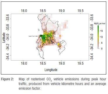
A model describing the number of vehicles and vehicle kilometres travelled in an hour during peak hours on each section of road was obtained from an emissions report for the City of Cape Town,10 and is based on vehicle count data. No public information is available on vehicle composition for the city, so an average emission factor was used, calculated from available vehicle types supplied by the Greenhouse Gas Protocol guidelines for emissions calculations,11 based on the US Environmental Protection Agency's (EPA) published values, and the Department for Environment, Food and Rural Affairs' (Defra) guidelines,12 which therefore assume an equal distribution of vehicles in each vehicle category. The average emission factor calculated was 347.01 g of per vehicle kilometre, with a standard deviation of 239.64 g of CO2 per km.
This emission factor converts vehicle kilometres into CO2 emissions. The total number of vehicle kilometres travelled in a particular pixel was calculated by rasterising the line object data from the supplied shape file on vehicle kilometres provided by the City of Cape Town, so that the sum of vehicle kilometres over all lines were equal to the sum of vehicle kilometres over all pixels. The proportion of vehicle kilometres allocated to a pixel was the same as the proportion of the length of the line which occurred inside the pixel. This was performed using the rgeos™ and raster14packages in R (a statistical software package).
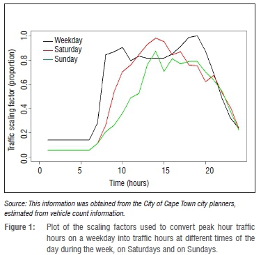
In addition to the model describing the distribution of vehicle kilometres on Cape Town roads during peak hours, scaling factors were also provided to describe the traffic intensity at different times of the day, both over weekdays and weekends. These hourly scaling factors were used to transform the peak time weekday vehicle kilometres to match with a particular day of the week and time, so that a spatially explicit time series could be created with an hourly time step from Monday through to Sunday (Figure 1).
Domesttc emissions
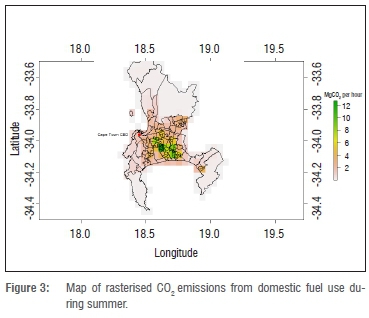
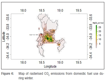
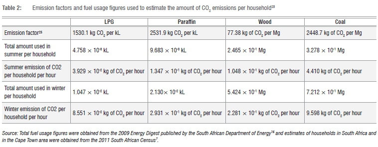
To obtain the emissions from domestic fossil fuel burning for lighting, cooking and heating, data on the number of households from the 2011 census and data on the amount of residential fuel usage from the 2006 and 2009 Energy Digests15,16 were used. The average amount of fuel usage per household was obtained by dividing the total fuel usage across the whole country by the number of households reported in the 2011 South African census (14 450 161). The average amount of fuel used per household was multiplied by the number of households in each pixel, and this value was scaled according to the proportion of fuel used for cooking, lighting and heating, where 75% of the annual heating fuel usage was assumed to take place during the winter months (March to August). It was assumed that 75% of the annual energy consumed was used for heating, 20% for cooking and 5% for lighting.
The population of Cape Town was subdivided into the different wards of the city, and these data were recorded as a shape file containing polygons of the wards and the associated population and household count. Using a similar method as for the vehicle line data, the polygon information was rasterised into pixel data so that the sum of the household counts over all the wards equalled the sum over all the pixels. The proportion of the household count that was assigned to each pixel was determined by the proportion of the polygon area located inside the pixel. This method can be extended to accommodate socio-economic data about the different wards used in our study, where the emissions from residential fossil fuel burning can be allocated based on income levels or electricity consumption because more affluent households will largely depend on electricity for heating, lighting and cooking. In order to better understand the discrepancies in household fuel usage, we have left this aspect for a future study.
industriai emissions from iisted activities
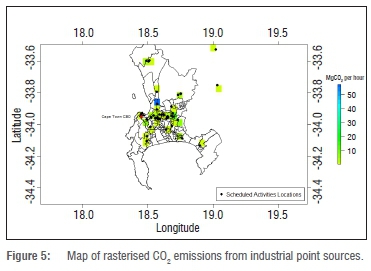
Under South Africa's Air Quality Act, industry must obtain an emissions licence to perform certain listed activities, and reporting of activity data for the purpose of emissions calculations is mandatory.17 The dominant industrial activities listed include ceramic processes, hydrocarbon refining processes, iron and steel processes, Macadam processes for asphalt production, and waste incineration processes, as well as electricity generation at gas turbine power plants.18 The initial approach was based on the methodology from Gurney2 for point source industrial emissions in the USA, where CO emissions were converted into CO2 emissions based on the ratio between CO and emissions factors for that industry. Because of the coarseness of the reported CO emissions, we were unable to break the emissions down into different processes for which CO could be converted into CO2 emission using the industry and process specific emission factors.
As an alternative, the reported fuel usage data for the top fuel users were converted directly into CO2 emissions by multiplying this fuel usage date with the Defra greenhouse gas emission factors.12 The fuel types that were considered included heavy fuel oil, coal, diesel, paraffin and fuel gas which were divided into liquid petroleum gas and refinery fuel gas. In the case of gas fuels, which were recorded in units of Nm3, the fuel usage was first converted into kWh, and then into CO2 emissions, where the calorific values were obtained from Rayaprolu19 so that Defra emission factors could be used. The point data were then aggregated into the required raster format through summing the emissions from each source in a pixel. This analysis only took into account emissions from fuel combustion, not process related emissions.
Airport and harbour emissions
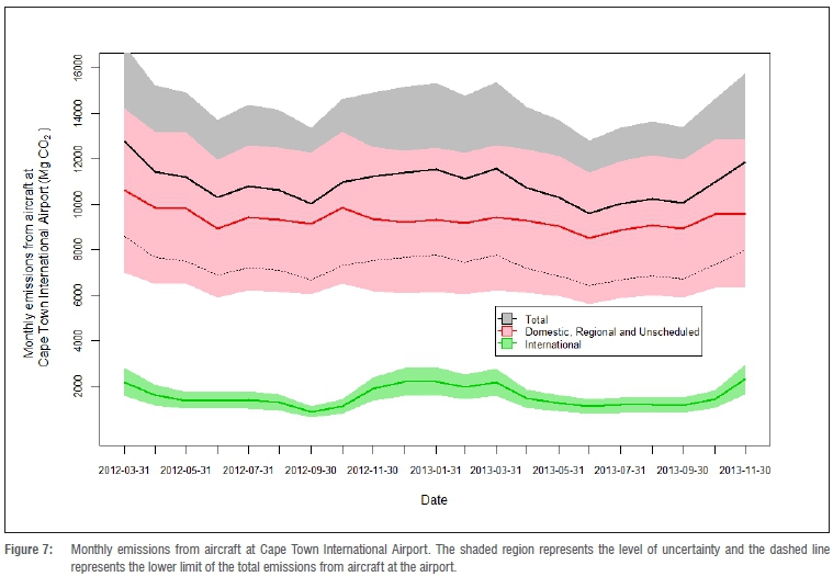
Emissions from aircraft are normally separated into the landing/takeoff cycle (LTO) and the cruise phase of the flight. The LTO part of flights at the Cape Town International Airport is allocated to the city's emissions, and divided evenly over the area which covers the airport. The Airports Company South Africa provides data on the number of aircraft movements, separated into domestic and international flights, for each month.20 The IPCC guidelines provide emission factors per LTO,21 separated into domestic and international flights. These emission factors were used to convert the monthly count of aircraft movements into CO2 emissions.
The monthly emission was then divided equally between days, but emissions were only allocated to the hours between 06:00 and 22:00, when most of the aircraft activity takes place at the airport. The average emission factor for the domestic fleet was reported to be 2680 kg of CO2 per LTO, and the average emission factor for the international fleet was 7900 kg of CO2 per LTO.
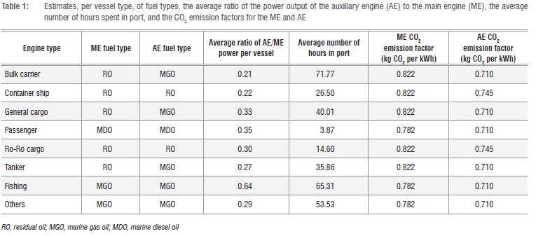
The National Ports Authority of South Africa22 publishes statistics on the harbour activity at the Cape Town Port on a monthly basis. The UK's Defra published a report on 2010 shipping emissions in the UK23 and this report was used as a guideline to obtain estimates of the average amount of time spent by a particular vessel type in port, the average power of the main engine (ME) and auxiliary engine (AE) of each vessel type, and the emission factors for each vessel type while at berth and performing manoeuvring activities in port. The guidelines provided the equation to convert the gross tonnage of a vessel into total ME power:

as well as the estimated proportion of power of the AE relative to the ME for a particular vessel type. The emission formula used is:

where E is the emission, T is the time in hours spent in port, ME is the power of the main engine, AE the power of the auxiliary engine, LF is the loading factor for a particular engine and EF is the emissions factor for a particular engine. At berth and while manoeuvring, vessels are expected to operate at 20% of the maximum continuous rating for main engine operation and at 45% of the maximum continuous rating of the auxiliary engine (Table 1).
As for airport emissions, the monthly estimates were divided between each day and each hour of the month, but no assumption was made regarding when the activity took place, so emissions were allocated to all hours of the day.
The monthly emission values from the airport or harbour were allocated to a polygon describing the shape of the airport or harbour respectively. The polygons were then rasterised using the same grid as for the previous emission fields. To obtain hourly emission estimates, the total emissions for the month were divided by the number of days in the month, and then divided by 24 to get the hourly emission value. In the case of airport emissions, the daily emissions were divided by 16 instead, because it was assumed that the bulk of aircraft activity took place from 06:00 until 22:00.
Uncertainty analysis
Uncertainty estimates are required, not only to show the reliability of the estimates, but the inverse modelling approach requires prior flux estimates as well as prior error estimates for the covariance matrix of the estimated fluxes.
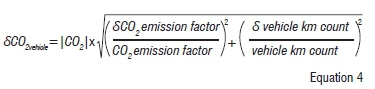
As no information was available on the error of the vehicle counts model, the nature of the data was used to obtain the estimate of uncertainty. The model provides the mean number of vehicle kilometres over a unit distance, and therefore it is likely that the data will follow a Poisson process, which implies that the variance of the estimate should be equal to the mean, and therefore the standard deviation equal to the square root of the mean. The CO2 emission is the product of this count in vehicle kilometres and the average CO2 emission factor, which has a standard deviation of 239.64 g of CO2 per kilometre. From error propagation laws, the error in the CO2 emission estimate will then be:
According to the Statistical Release of the 2011 South African census, the omission rate for the census questionnaire was approximately 15%.7 The average fuel usage data per household was calculated by dividing the total annual amount of fuel sold by the number of households. No data were available for the difference in fuel usage between households. Therefore, to account for the missing source of uncertainty, the omission rate was elevated to 30%, double that of the omission rate, and this used as the estimate of the uncertainty in domestic emissions.
A report was published for the UK on the treatment of uncertainties of greenhouse gas emissions,24 which provided estimates of activity data error and emission factor error under each fuel type for industrial sources. As the CO2 emission at a particular point source is calculated as:

Error propagation techniques can be used to determine the uncertainty of the final estimate as:
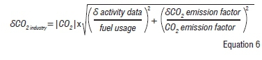
where δ is the uncertainty value. The uncertainties provided are expressed as proportions of the amount of fuel use and of the size of the emission factor, therefore the uncertainty for the final CO2 emission can be simplified to:
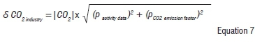
for the reported fuel usage data and for the emission factor respectively for a given fuel type.
The aircraft count data are assumed to be without error, and therefore the error will be contained in the emission factors. The standard deviations of the emission factors of individual aircraft used to calculate the average emission factor for the domestic and international fleet were used to determine the uncertainty of the aircraft emissions. This was found to be 34% of the mean emission factor for the domestic fleet and 28% for the international fleet.21
As for the aircraft data, the counts of different ships in the harbour are assumed to be correct. Therefore, the error is assumed to lie in the emission factors for the different vessel types. From the Defra UK shipping inventory guide,23 the assumed errors for berth and manoeuvring activities in the port are 20% and 30%, respectively. Therefore, to ensure a conservative estimate, the error is assumed to be 30% of the estimate.
Total emissions
Once the layers for each emission source type are obtained, the total emissions for a particular hour or any particular period can be obtained by summing the raster layers, where the appropriate scalar manipulations have been performed, such as multiplying the vehicle emission layer by the appropriate scaling factor for the day of the week and time of day. In order to be able to obtain the error estimates for each pixel, the uncertainties need to be expressed as variances instead of standard deviations, and then the variances for each of the source emission estimates in a pixel can be summed to obtain the total variance, which can then be converted back into a standard deviation by taking the square root of the variance.
Fossil fuel product comparison
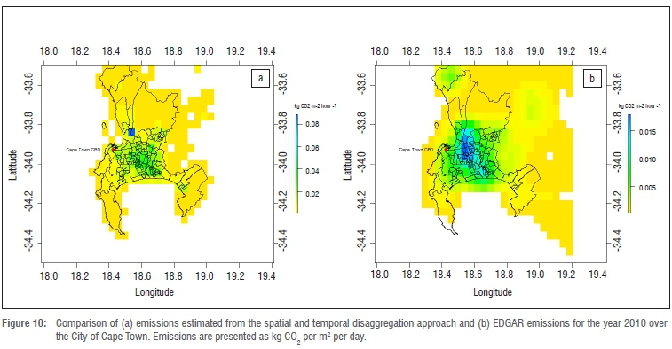
To determine if the emissions estimated in this study are reasonable, the emissions for a weekday in March 2012 were compared with the EDGAR product. The spatial distributions of the emissions were mapped for each of the products, and the total emissions for the domain of Cape Town were calculated and compared between the two products.
Results and discussion
Road transport vehicle emissions
The rasterised vehicle emissions during peak hour traffic showed the concentration of emissions around the city centre of Cape Town and over the highway routes leading into the city from the suburban areas. Using the equation for uncertainty in the emission estimates, the pixel with the largest emission estimate of 19.74 Mg CO2 per hour had an error estimate of 16.45 Mg CO2 per hour. The error estimate was 83% of the emission estimate. The error in the vehicle emissions was expected to be large as there was a great deal of uncertainty in the average emission factors, with factors ranging from 100.1 g to 1034.6 g of CO2 per kilometre.
Domestic emissions
Residential emissions from domestic fuel use were distributed over the suburban areas around Cape Town, as expected (Figures 3 and 4). Owing to the assumption that more fuel was used for heating purposes in the winter months, the maximum levels of emissions during summer were approximately half of what was consumed during the winter months (Table 2). The largest emission estimate for a pixel was 27.7 Mg CO2 per hour during the winter months. The error of the estimate, using the assumed 30% error rate, was 8.3 Mg CO2 per hour.
Industrial emissions from scheduled activities
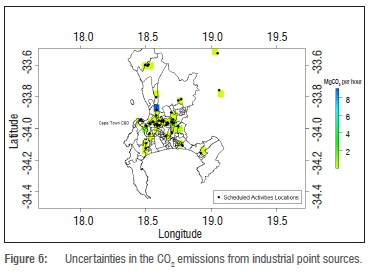
The emissions resulting from industrial processes are distributed slightly away from the CBD towards the outskirts of the city centre, spreading outwards towards the city boundaries (Figure 5). The largest per pixel emission was 57 Mg CO2 per hour, with an error value of 9 Mg CO2 per hour, which is 16% of the mean value (Figure 6).
The advantage of obtaining the CO2 emissions by using the fuel data compared to converting the CO emissions for different industries is that the error estimates are much smaller, as the fuel data have a much smaller associated error than estimated CO emissions for a particular industry. The disadvantage of the fuel data approach is that emissions from process-related activities are ignored, but would be included if the total CO emissions were converted into CO2 emissions. Both the fuel data and the CO emission data are difficult to access and rely on accurate reporting from the industrial firms.
Airport and harbour emissions
The emissions from aircraft at the airport are on average 10 890 Mg of CO2 a month, with higher emissions during November to January when air traffic increases into the city (Figure 7). The average hourly emission from aircraft at the airport is 15.1 Mg of CO2. This analysis does not include the emissions from point sources or ground vehicles at the airport and will require a count of each aircraft type arriving at the airport. The Defra guidelines for aircraft emissions supply the average amount of time each ground unit spends in operation per LTO cycle for a particular aircraft type, and these estimates could be used to determine emissions from ground vehicles at the airport.
The total emissions from shipping vessels in the Cape Town harbour, at berth and during manoeuvring procedures, are on average 4171.6 Mg of CO2 per month (Figure 8), which is approximately 5.8 Mg of CO2 per hour. Emissions take a dip during the mid-winter months, when the seas around Cape Town are particularly rough and storms are prevalent.
Total emissions
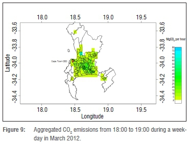
To demonstrate the aggregation of the different source emission layers, the total emissions estimated for a weekday in March 2012 at 18:00 were obtained. The industrial emissions and power station emissions were assumed to take place at all times, so the same layer would be used regardless of which hour was of interest. March falls into the winter period, so the winter domestic emission layer was used, and because it was a weekday at 18:00, no scaling was necessary for the vehicle emissions layer. The airport and harbour emissions for March 2012 were used. The monthly value was divided equally between all hours of the month for harbour emissions and divided evenly between all days and the hours from 06:00 to 18:00 in the case of the airport emissions. These layers were summed and the resulting emission layer was mapped (Figure 9).
Fossil fuel product comparison
A comparison with the EDGAR 0.1°x0.1° product over Cape Town revealed a similar allocation of CO2 emissions for different areas, but with the EDGAR product providing a more smoothed product (Figure 10). The total emissions calculated in this study were strongly influenced by the large point source industrial emitters. The total emission of CO2 during a weekday in March over the full spatial domain of Cape Town was 9 252 883 kt. Calculated from the EDGAR data, which is provided in kg CO2 per m2 per second, the total emission for the same area would be 7 574 559 kt. The EDGAR data are available until 2010, therefore there is a 2-year lag between the two products compared. The EDGAR data provided are also an average value for the year, and therefore it is not surprising that our study estimated a 22% higher CO2 emission than that considered for a typical weekday in March 2012.
Discussion and conclusions
The results for the City of Cape Town show that through the use of publicly available data and reported data on activity and population levels around the city, it is possible to obtain a spatially and temporally explicit inventory of emissions. The most challenging of the sectors was the industrial sector, for which data at the required resolution are not always available in adequate detail. These fossil fuel emission estimates are essential to run an atmospheric inversion for the city to obtain improved estimates of the total CO2 fluxes occurring in and around the city.
These estimates can be improved by obtaining detailed fleet data for vehicle, aircraft and shipping vessel movements, as the emission factors differ significantly among different fleet types. Domestic emissions estimates can be improved by using Cape Town specific surveys on the average fuel use quantities, and distinguishing these surveys between different households depending on domicile type, as those homes with better amenities are less likely to rely on solid and liquid fuels for cooking, heating and lighting. The estimates of the emissions from the power stations and industrial sources could be improved if more detailed fuel usage and specific process data were available for each facility included in the assessment. It may be useful for South Africa to publish a similar document to the one Defra publishes for the UK, with South Africa specific emission factors, to increase accuracy and so that emission estimates by different professionals can be standardised for South Africa. A comparison with a global benchmark emissions product revealed that the proposed method, making use of the currently available usage data, provides reasonable estimates of CO2 emissions, which would be further improved if South Africa specific emission factors were used.
The results obtained through this process will provide important inputs required for an atmospheric inversion study, relying on observations from a network of CO2 measurement equipment placed around the city. A similar approach as described in this paper will be used to disaggregate the national emissions, to provide coarser estimates of CO2 emission from fossil fuel combustion, which will then be used in a national inversion study. The best placement of new measurement sites for the observation of CO2 sources and sinks at a national level has already been determined through an optimal network design.26 Improving the knowledge of the South African CO2 budget will help to reduce the uncertainty of the global estimates of sources and sinks, as southern Africa is usually a large source of error in global inversions, because of Africa's general under-sampling of greenhouse gas concentration measurements.27
Acknowledgements
This work was supported by parliamentary grant funding from the Council of Scientific and Industrial Research, South Africa, project number JECOS81. We thank Karen Small of the Strategic Development Information and Geographic Information System Department of the City of Cape Town for providing the Western Cape census shape files, and Sarah Ward of the City of Cape Town for providing access to emission data collected by the City of Cape Town.
Authors' contributions
A.N., the main author, was responsible for data acquisition, data processing, statistical analysis, model development and writing of the manuscript. R.J.S. provided scientific advice and E.F. was involved with data provision and processing and provided scientific advice.
References
1. Eggleston HS, Buendia L, Miwa K, Ngara T, Tanabe K, editors. IPCC Guidelines for National Greenhouse Gas Inventories. Tokyo: IGES; 2008. [ Links ]
2. Gurney KR, Mendoza DL, Zhou Y Fischer ML, Miller CC, Geethakumar S, et al. High resolution fossil fuel combustion CO2 emission fluxes for the United States. Environ Sci Technol. 2009;43(14):5535-5541. http://dx.doi.org/10.1021/es900806c [ Links ]
3. Janssens-Maenhout G, Pagliari V, Guizzardi D, Muntean M. Global emission inventories in the Emission Database for Global Atmospheric Research (EDGAR) - Manual (I). Gridding: EDGAR emissions distribution on global gridmaps. Luxembourg: European Union; 2012. p. 33. [ Links ]
4. Rayner PJ, Raupach MR, Paget M, Peylin P Koffi E. A new global gridded data set of CO2 emissions from fossil fuel combustion: Methodology and evaluation. J Geophys Res. 2010;115:D19306. http://dx.doi.org/10.1029/2009JD013439 [ Links ]
5. Asefi-Najafabady S, Rayner PJ, Gurney KR, McRobert A, Song Y Coltin K, et al. A multiyear, global gridded fossil fuel CO2 emission data product: Evaluation and analysis of results. J Geophys Res Atmos. 2014;119:10213-10231. http://dx.doi.org/10.1002/2013JD021296 [ Links ]
6. Gurney KR, Razlivanov I, Song Y Zhou Y Benes B, Abdul-Massih M. Quantification of fossil fuel CO2 emissions on building/street scale for a large U.S. city. Environ Sci Technol. 2012;46(21):12194-12202. http://dx.doi.org/10.1021/es3011282 [ Links ]
7. Statistics South Africa. Census 2011 statistical release - P0301.4. Pretoria: Statistics South Africa; 2011. [ Links ]
8. City of Cape Town. State of energy and energy futures report. Cape Town: City of Cape Town; 2011. Available from: http://www.capetown.gov.za/en/EnvironmentalResourceManagement/publications/Documents/ State_of_Energy _+_Energy_Futures_Report_2011_revised_2012-01.pdf [ Links ]
9. Eskom. Generating electricity at a nuclear power station: Fact sheet revision 8 [document on the Internet]. c2013 [cited 2014 Jan 16]. Available from: http://www.eskom.co.za/AboutElectricity/FactsFigures/Documents/NU_0001NuclearEnergyBasic CycleRev6.pdf [ Links ]
10. Cambridge Environmental Research Consultants. Compilation of emissions inventory and preliminary air quality monitoring for Cape Town. Report no. FM865/R5/12. Cape Town: City of Cape Town; 2012. [ Links ]
11. Greenhouse Gas Protocol. Calculating CO2 emissions from mobile sources [homepage on the Internet]. c2005 [cited 2014 Jan 16] Available from: http://www.ghgprotocol.org/files/ghgp/tools/co2-mobile.pdf [ Links ]
12. UK Department for Environment, Food and Rural Affairs (Defra). Government GHG conversion factors for company reporting: Methodology paper for emission factors. London: Crown; 2013. Available from: https://www.gov.uk/government/uploads/system/uploads/attachment_data/file/224437/pb13988-emission-factor-methodology-130719.pdf [ Links ]
13. Bivand R, Rundel C. Rgeos: Interface to Geometry Engine - Open Source (GEOS). R package version 0.3-2 [program on the Internet]. c2013 [cited 2014 Aug 28]. Available from: http://CRAN.R-project.org/package=rgeos [ Links ]
14. Hijmans RJ. Raster: Geographic data analysis and modelling. R package version 2.1-49 [program on the Internet]. c2013 [cited 2014 Aug 28]. Available from: http://CRAN.R-project.org/package=raster [ Links ]
15. South African Department of Minerals and Energy. Digest of South African energy statistics. Pretoria: Department of Minerals and Energy; 2006. Available from: http://www.energy.gov.za/files/media/explained/2006%20Digest%20PDF%20version.pdf [ Links ]
16. South African Department of Energy. Digest of South African energy statistics. Pretoria: Department of Energy; 2009. Available from: http://www.energy.gov.za/files/media/explained/2009%20Digest%20PDF%20version.pdf [ Links ]
17. National Environment Management: Air Quality Act, No. 39 of 2004. Government Gazette. 2005 Feb 24; vol. 476, no. 27318. [ Links ]
18. Eskom. Ankerling and Gourikwa gas turbine power stations fact sheet: Revision 6. Johannesburg: Generation Communication; 2013. Available from: http://www.eskom.co.za/AboutElectricity/FactsFigures/Pages/Facts_Figures.aspx [ Links ]
19. Rayaprolu K. Boilers: A practical reference. New York: Taylor and Francis; 2013. p. 181-183. [ Links ]
20. Airports Company South Africa (ACSA). Aircraft statistics [document on the Internet]. No date [cited 2014 Jan 13]. Available from: http://www.acsa.co.za/airports/cape-town-international/statistics/aircraft [ Links ]
21. Intergovernmental Panel on Climate Change (IPCC). Good practice guidance and uncertainty management in national greenhouse gas inventories. Montreal: IPCC; 2000. p. 93-102. Available from: http://www.ipcc-nggip.iges.or.jp/public/gp/english/ [ Links ]
22. Transnet National Ports Authority, South Africa. Summary of cargo handled at ports of South Africa [homepage on the Internet]. c2010 [cited 2014 Jan 16]. Available from: http://www.transnetnationalportsauthority.net/DoingBusinesswithUs/Pages/Port-Statistics.aspx [ Links ]
23. UK Department for Environment, Food and Rural Affairs (Defra). UK ship emissions inventory. Final report. London: Crown; 2010. Available from: http://uk-air.defra.gov.uk/assets/documents/reports/cat15/1012131459_21897_ Final_Report_291110.pdf [ Links ]
24. UK Department for Environment, Food and Rural Affairs (Defra). Treatment of uncertainties for national estimates of greenhouse gas emissions [homepage on the Internet]. c2013 [cited 2014 Mar 25]. Available from: http://uk-air.defra.gov.uk/reports/empire/naei/ipcc/uncertainty/contents.html [ Links ]
25. UK Department for Environment, Food and Rural Affairs (Defra). 2012 Guidelines to Defra / DECC's GHG conversion factors for company reporting. PB 13773. London: Crown; 2012. Available from: https://www.gov.uk/government/uploads/system/uploads/attachment_data/file/69554/pb13773-ghg-conversion-factors-2012.pdf [ Links ]
26. Nickless A, Ziehn T, Rayner PJ, Scholes RJ, Engelbrecht F. Greenhouse gas network design using backward Lagrangian particle dispersion modelling -Part 2: Sensitivity analyses and the South African test case. Atmos Chem Phys. 2015:2051-2069. http://dx.doi.org/doi:10.5194/acp-15-2051-2015 [ Links ]
27. Denman KL, Brasseur G, Chidthaisong A, Ciais P Cox PM, Dickinson RE, et al. Couplings between changes in the climate system and biogeochemistry. In: Solomon S, Qin D, Manning M, Chen Z, Marquis M, Averyt KB, et al., editors. Climate change 2007: The physical science basis. Contribution of Working Group I to the fourth assessment report of the Intergovernmental Panel on Climate Change. Cambridge: Cambridge University Press; 2007. p. 499-587. [ Links ]
 Correspondence:
Alecia Nickless
Global Change and Ecosystem Dynamics, Natural Resources and the Environment
Council for Scientific and Industrial Research
PO Box 395, Pretoria 0001
South Africa
Email: alecia.nickless@phc.ox.ac.uk
Received: 05 Nov. 2014
Revised: 10 Feb. 2015
Accepted: 15 Feb. 2015

