RESEARCH ARTICLE

 

Studies on CO variation and trends over South Africa and the Indian Ocean using TES satellite data

 

 

Abdoulwahab M. Toihir^{I, II}; Sivakumar Venkataraman^II; Nkanyiso Mbatha^III; Sivakumar K. Sangeetha^IV; Hassan Bencherif^I; Ernst-Günther Brunke^III; Casper Labuschagne^III

^IAtmosphere and Cyclones Laboratory, University of Réunion Island, Saint Denis, Réunion Island, France
^IISchool of Chemistry and Physics, University of KwaZulu-Natal, Durban, South Africa
^IIISouth African Weather Service, Stellenbosch, South Africa
^IVSchool of Geography and Environmental Sciences, University of KwaZulu-Natal, Durban, South Africa

Correspondence

 

 

---

ABSTRACT

In this study, we used measurements from the tropospheric emission spectrometer aboard the Earth Observing System's Aura satellite over South Africa, Madagascar and Reunion Island to investigate variations and trends in tropospheric carbon monoxide (CO) over 5 years, from 2005 to 2009, and at 47 pressure levels from 1000 hPa to 10 hPa. We believe that the study is the first of its kind to address the use of space-borne data for CO distribution over southern Africa. Maximum CO was recorded during spring and minimum during summer. Positive anomalies were identified in 2005 and 2007 during the spring and negative anomalies in the beginning of the year (especially in 2006, 2008 and 2009). The estimated trends based on a linear regression method on inter-annual distribution predicted a decreasing rate of 2.1% per year over South Africa, 1.8% per year over Madagascar and 1.7% per year over Reunion Island. The surface CO measurements made at Cape Point station (34.35°S, 18.48°E) showed an average decline of 0.1 ppb per month, which corresponded to 2.4% of the average annual mean for the studied period. The observed decrease in CO was linked to the La Nina event which occurred in 2006 and 2008 and a declining rate of biomass burning activity in the southern hemisphere over the observation period. TES measurements are in agreement with ground-based measurements and can be used with confidence to complement CO measurements for future analyses over the southern tropics and middle latitude.

Keywords: Aura satellite; remote sensing; carbon monoxide; vertical profile; annual trend

---

 

 

Introduction

Carbon monoxide (CO) is the subject of our study and it is produced by incomplete combustion of hydrocarbons like fossil fuel, biofuel and methane (CH₄) with insufficient oxygen, which prevents complete oxidation to carbon dioxide (CO₂). CO is a reactive gas that regulates the concentrations of several greenhouse gases in the atmosphere (e.g. ozone, methane and carbon dioxide) and plays an important role in tropospheric photochemical processes. Its chemistry is relatively simple and lifetime relatively long (from weeks to months, depending on the region and on the season), enough for one to follow pollutant movements and dispersions on a regional and global scale.¹ Thus, the present study on tropospheric distribution and variability of CO is important for monitoring and evaluating photochemical processes and transport of tropospheric traces gases.

There are different remote sensing instruments currently in use for retrieving CO information from various atmospheric layers. Among the means of remote sensing, observations include measuring devices from ground-based instruments on board commercial aircraft and high technology instruments aboard satellites. Within the framework of observations by satellite, Earth Observing System (EOS) is the biggest world programme for earth monitoring and observation. This programme coordinates several polar-orbiting and low inclination satellites measuring atmospheric parameters and particles at local and global scale. Among the EOS satellites, there is EOS Aura, which contains the tropospheric emission spectrometer (TES) instrument measuring carbon monoxide in the atmosphere.^2,3 With good spatial coverage, satellite measurements offer the best method for providing CO measurements over the globe; however, their height and temporal resolution is poor in comparison to most ground- based instruments. It is therefore necessary to compare the satellite measurements with ground-based and/or mathematical numerical models.

A previous study by Kopacz et al.⁴ from February to April 2001, used the atmospheric chemical transport model in order to validate and compare Asian CO sources detected by Measurements of Pollution in the Troposphere (MOPITT). Similarly, Luo et al.⁵ used a simulated concentration of CO from the Global Earth Observation System (GEOS) chemistry global three dimensional models as a time varying synthetic atmosphere in order to demonstrate and assess the capabilities of TES nadir observations. It is important to consider that two instruments from the same programme may not provide identical concentrations of tropospheric CO due to their different characteristics and modes of observation. A previous comparison study between TES and MOPITT CO measurements showed significant differences in the lower and upper troposphere, which led to a review of the instruments and to adopt adjustment and correction methods in order to improve the agreement between them.⁶ Heald et al.⁷ illustrated that MOPITT and Transport and Chemical Evolution over the Pacific aircraft programme (TRACE-P) CO observations are independently consistent to provide information about the Asian CO emission sources, with the exception of Southeast Asia. Richards et al.⁸ performed a study on TES CO measurements that was assimilated into the global chemistry transport model. Their work has shown that the assimilated data have a good agreement with MOPITT observations, especially at higher pressure levels in the southern tropics region. In some cases, CO measurements from different instruments are combined in order to estimate a global emission with accurate quantification. This is the case with an adjoining inversion method of multiple satellites (MOPITT, Atmospheric Infrared Sounder (AIRS), Scanning Imaging Absorption spectrometer for Atmospheric Chartography (SCIMACHY) and TES) used by Kopacz et al.⁹ to investigate global carbon monoxide distribution sources with a high spatial resolution (4°x5°) and a monthly temporal resolution. A comparative study of CO total column from three satellites' sensors - AIRS, MOPITT and Infrared Atmospheric Sounding Interferometer (IASI) - and two ground-based spectrometers, one in central Moscow and the other in its suburb Zvenigorod, was made during summer when forest fires are expected; the results revealed that all of the instruments were in good agreement during fires and when there were no forest fires.¹⁰

Surveys on air pollution have previously been made in the Indian Ocean region using remote sensing tools such as the AIRS instrument, which investigated carbon monoxide variation over the Malaysian peninsula that had originated from Indonesian forest fires.¹¹ However, no similar scientific studies on carbon monoxide investigations using TES measurements have been performed. Previous studies have shown that the west southern Indian Ocean region seasonally receives CO from Africa and South America^9,12, south western Asia¹² and India^9,13. However, the African and southern American contributions were observed below 11 km, while the south western Asia contribution was observed in the upper troposphere.¹² In addition, these previous studies have reported maximum CO in Africa and the Indian Ocean region during the biomass burning period from July to November. Khalil and Rasmussen¹⁴ reported that from 1988 to 1992, the global CO began to decrease at a rate of 2.6±0.8% per year, probably due to reduction in tropical biomass burning. Similarly, Novelli et al.¹⁵ confirmed that CO emissions have significantly reduced from 1990, especially in the southern hemisphere, whereas in the northern hemisphere, CO decreased at an average rate of 6.1% per year from June 1990 to June 1993. Zeng et al.¹⁶ reported that the trend of CO in the southern hemisphere from 1997 to 2009 was negative due to a decline in industrial emissions.

The present study is focused on using TES data in order to investigate the inter-annual CO total column distribution and trends, as well as to explain monthly and seasonal CO vertical profiles over South Africa and the Indian Ocean (Madagascar and Reunion Island) region. These two regions have different climatology but have several similarities due to their geographical proximity. The present work does not only provide insight into CO distributions within the region under investigation, but also explores the capability of the TES instrument to complement the CO measurement in the geographic zones. We also validate the TES data by performing a comparison between the TES measurements recorded at ~1000 hPa when the satellite overpasses closest to the Cape Point Global Atmosphere Watch (GAW) station (34.35°S, 18.48°E). The ambient surface CO measured at Cape Point during the TES overpasses are used for comparative purposes.

 

Data sources

TES instrument

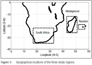
The tropospheric emission spectrometer (TES) is an imaging infrared Fourier transform spectrometer in polar sun-synchronous orbit aboard the EOS Aura satellite, launched on 15 July 2004. TES is dedicated to measure from nadir and limb, viewing the infrared radiance emitted by the earth's surface, atmospheric gases and particles from space. TES measurements are routinely performed from 650 to 3050 cm¹ spectral range (3.3-15.4 μηι).² The apodised spectral resolution for standard TES observation is 0.1 cm¹; however, finer spectral resolution (0.025 cm¹) is used during special observations. In this present work, we are interested only in CO observation from nadir viewing in which the CO information is retrieved from space on the 2000-2200 cm¹ absorption band.³ Nadir observations have a footprint of 5 km X 8 km, averaged over detectors in which each pixel covers a spatial resolution of 0.5 km X 5.3 km. TES uses both the natural thermal effects issued by the atmosphere and sunlight reflected from ground, allowing night and day observations. The routine observations performed by TES are referred to as 'a global survey'. A global survey is run every other day on a predefined schedule and collects 16 orbits (~26 h) of continuous data. A series of repetitive units, referred to as a sequence, is performed in each orbital track. The possible maximum number of sequences per run is 72 for 26 h of observation. Thus, 1152 profiles are provided at global scale during these 26 h of observation. For the purpose of the present study, only profiles recorded for overpasses over South Africa, Madagascar and Reunion Island have been selected and used. The geographic locations of these three selected sites are indicated in Figure 1. (For further information on the TES instrument, the reader may visit the web page http://tes.jpl.nasa.gov.)

 

 

TES data

The data retrieval processing was performed in the selected areas for each day when a global survey was made. The number of profiles retrieved during a global survey varied between 0 and 16 profiles, depending on the extension of the observed area with respect to the satellite location during the observation period. It is worth noting that nadir observation covers a field of view of 5 km χ 8 km. The considered geographical delimitations for the selected sites are shown in Figure 1 and Table 1. However, during observation time, there is a possibility that no observations were obtained in one or two of the selected areas (South Africa, Reunion and Madagascar).

 

 

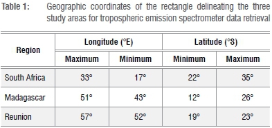
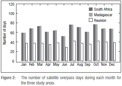
Figure 2 shows the number days of observation recorded in each area with respect to the month during the study period (01 January 200531 December 2009). Figure 2 indicates that South Africa and Madagascar have more observations, probably because of their larger size when compared to Reunion Island. Nevertheless, the number of observations over Reunion Island was found to be acceptable for the purpose of this study. It is worth noting that the number of days recorded at Reunion Island for a specific month (e.g. January 2007) was between 2 and 10, whilst in South Africa and Madagascar, the frequency was between 3 and 16 days (except in June 2005 when no CO measurements from TES were received).

 

 

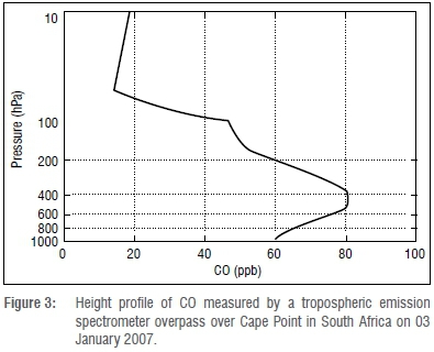
Each TES mean daily vertical profile is composed of 47 pressure levels between 1000 hPa and 10 hPa and deducted by averaging daily vertical footprints recorded over the site during the observation. Figure 3 shows an example of a vertical TES CO profile recorded for 03 January 2007 during a close satellite overpass of Cape Point (34.35°S, 18.48°E) in South Africa. It illustrates CO mixing ratio values of ~59.5 ppb at ground level ~1000 hPa and the maximum is observed in between the 500 and 400 hPa pressure levels. The CO mixing ratio continues to decrease above 400 hPa and reaches a minimum value of ~14.8 ppb at around 51 hPa. The decrease is significant especially above 100 hPa (above the troposphere layer).

 

 

Trace analytical RGA-3 instrument

The trace analytical RGA-3 is an analyser used to measure CO. The different chemical components of an atmospheric sample are separated by gas chromatography (GC) utilising a column filled with a molecular sieve that is specific to Co retention. Upon heating, the eluted species are directed to a detector, which contains mercuric oxide (HgO). The RGA-3 instrument characteristics and operator mode are well documented by Hammer¹⁷. In this study, a trace analytical RGA-3 instrument was used for surface CO measurements at Cape Point in South Africa, which is one of South African Weather Service's long-term trace gas measurement stations.¹⁸

Cape Point station and CO measurements

The Cape Point global atmospheric watch laboratory (34.35°S, 18.48°e) is situated approximately 60 km directly south of Cape Town, and is located on a coastal cliff 230 metres above sea level within a nature reserve. It experiences moderate temperatures - dry summers impacted by occasional biomass burning episodes from the surrounding areas and increased precipitation during the austral winter months. Various wind systems (from both the marine and continental sectors) constitute the annual climatology. The observatory has been operational since 1978 and continues to provide long-term trace gas data - including CO. Cape Point station is managed by the South African Weather Service and coordinated by the GAW network through the World Meteorological Organization.

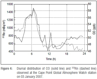
The station is predominantly exposed to maritime air masses that are derived from the southwestern and southeastern Atlantic Ocean regions, which constitute background conditions.^18,19 The daily average Cape Point CO mole fractions are calculated from 12-min values made by a RGA-3 trace analytical instrument and compiled to yield 30-min averages. Figure 4 presents the Cape Point CO measurements recorded on 03 January 2007 during such a specific overpass. In addition, Radon-222 (²²²Rn), which is an excellent tracer for air mass origin, was used to characterise the air type on the day under scrutiny. Generally, ²²²Rn >1200 mBq/m³ is associated with continental air masses, while ²²²Rn <250 mBq/m³ is representative of baseline conditions with the oceanic air component dominating.¹⁹ It can be seen from Figure 4 that on this date, CO mole fractions (solid line) varied between 46 and 60 ppb (right axis), whilst ²²²Rn (dash line) fluctuated between 372 and 1485 mBq m³ at the same time. These conditions primarily reflect continental and mixed air masses¹⁹ with a small marine component after 20:30 (local time). CO and ²²²Rn also correlate very well (Figure 4) revealing common source regions on this occasion. A strong continental air signal was evident during the early morning hours (04:00 to 07:30) when ²²²Rn exceeded 1200 mBq/m³, while later in the day (10:00 till midnight), ²²²Rn levels fluctuated between 400 and 600 mBq/m^3, typically reflecting mixed air mass conditions (marine air with some entrainment of continental air) in response to a varying wind regime. The ²²²Rn is used in this work to characterise the observation day in which the surface CO recorded at Cape Point station was contaminated by continental air mass. The present study uses only the daily average data from Cape Point uncontaminated by continental air mass to compare with the TES daily data recorded at 1000 hPa overpass over Cape Point.

 

 

Data analysis

The CO daily profile obtained from TES observation recorded overpasses over South Africa, Madagascar and Reunion have been analysed in order to examine the CO regional and seasonal distribution and to estimate its inter-annual trend. Thus, the statistical descriptive method is adopted and the inter-annual trend is estimated based on linear regression analysis. Prior to analysing the climatological, seasonal and monthly variations of CO over the selected regions, we first established a comparison of TES data with the ground-based measurements.

In order to facilitate a meaningful inter-comparison between TES and Cape Point CO data, the air mass block (vertical and lateral dimension) over the Cape Point region as seen by TES should be as homogeneous as possible. If this is not the case, the likelihood of TES seeing the same CO air mixture as the Cape Point laboratory will be greatly reduced, especially during pollution episodes. However, when southerly onshore maritime air flow regimes exist, the conditions for inter-comparisons are optimal. Such maritime air flow systems are easily identified using ²²²Rn data.¹⁹ According to Brunke et al.¹⁹ and in order to classify the air masses over Cape Point during TES overpasses, only CO data during which the daily average ²²²Rn level did not exceed 250 mBq/m³ were selected for inter-comparison.

The TES profiles selected were those recorded between 34.35±0.5°S and 18.48±0.5°E. The daily selected value of TES was that registered at -1000 hPa (ground level) while the daily value of surface based CO was computed from higher resolution in-situ measurements made at the Cape Point station. Comparison between the TES and ground-based values were performed each day when TES and filtered ground-based data were available. A total of 184 TES profiles were recorded over Cape Point during the period of observation (January 2005-December 2010). However, only 52 profiles were recorded on days in which ground-based data was not contaminated by continental air mass. Finally, the comparison was achieved on these 52 days of observation. The comparison indexes used were the relative differences, mean bias error, absolute root mean square and correlation coefficient R²between TES and ground-based observations. The CO relative difference (RD) between TES and Cape Point observed for a given day d was calculated with the following expression:

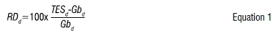
where Gb_d and TES_d represent the daily values of ground-based and TES data, respectively. The mean bias error was taken as the average value of relative difference. The mathematical expression of the mean bias error (MBE) is:

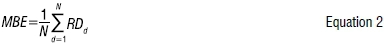
where N represents the number of day-pairs between the TES and Cape Point measurements. The correlative coefficient and absolute root mean square between the two observations was assessed using the linear regression method.

 

Results and discussion

Comparison between ground-based measurements and TES overpasses

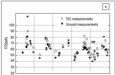
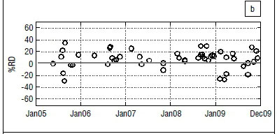
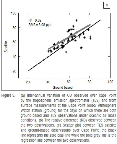
The comparison between TES satellite and ground-based observations were performed in order to validate the satellite measurements over Cape Point station. Methodology used for data processing were given in the precedent sections while the results are presented here. Figure 5a shows temporal variations of CO measured at the Cape Point station (black crosses) and from TES (grey circles) for the time period from 01 January 2005 to 31 December 2009. In Figure 5b, the figure is superimposed with the relative difference between the two observations with respect to the ground-based measurement. It is apparent that the seasonal and inter-annual variation between the surface-based and satellite observations are found to be consistent and the obtained relative difference is within ±40%. Correlation between the two observations is given in Figure 5c. The correlation coefficient R² obtained between TES and ground-based measurements was evaluated and found to be around 0.61. Furthermore, Figure 5c shows a regression linear line (grey colour line) above the unit slope line (black line), indicating an overestimation of TES measurement with respect to ground-based. However, the obtained mean bias error is assessed at around 6.6% and the absolute root mean square recorded between the two observations is estimated to be less than 8.1 ppb. This difference is in part due to the different instrumental characteristics. TES uses an infrared high-spectral resolution Fourier transform spectrometer whilst at the Cape Point Observatory, the instrument is a RGA-3 trace analytical gas chromatograph. The difference in the time of observation may also explain the different values observed (one observation per day for TES and 48 individual 30-min observations in the case of surface measurements). Even the spatial resolution of TES (0.5 km x 5.3 km) can play a role in the observed differences between TES and ground-based measurements. However, the difference in measurements has not modified the overall variations within the temporal structure for the annual distribution between the TES Aura satellite and surface observations. Hence, we propose that it is possible to use TES data to study CO distribution for other localities.

 

 

The climatology of CO observed over the three regions

The monthly climatological profile was deduced by averaging daily vertical profiles recorded during the month, irrespective of the year. The monthly variations of TES CO measurements over the three regions during 5 years (2005-2009) are plotted in Figure 6. Over the three selected regions, CO measurements show a high variability in the free troposphere between 850 hPa and 150 hPa. It was found that the CO mixing ratio varied between 55 ppb and 120 ppb from surface to ~100 hPa; thereafter, it showed linear variations, mostly decreasing over height and reaching less than 20 ppb at 50 hPa. The maximum value was observed during spring when maximum bushfires and biomass burning are reported in southern Africa and adjacent regions.^9,11-13,20

 

 

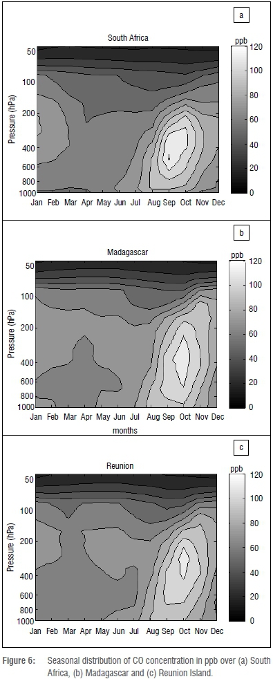
The minimum value of CO mixing ratio was observed during the summer period. This period was also marked by high humidity and high activity of UV (ultraviolet) radiation in the southern tropic and subtropics region that led to production of radical hydroxyls (OH) from ozone photolysis.²¹ Reaction with OH constitutes the primary sink for CO in the troposphere and consequently, the seasonal cycle of CO is primarily driven by the OH radical.^21,22

It is worth noting that tropospheric carbon monoxide is produced essentially around the atmospheric boundary layer. The rather elevated quantity observed in the free troposphere between 850 hPa and 150 hPa is due to large-scale air mass transport and vertical convection from the free troposphere to tropopause. During this upward movement, CO reacts with OH to produce other chemical species such as CO₂ and hydrogen. Alternatively, it can also be oxidised to CO₂ and ozone (O₃) following specific reactions.²² This could be one of the reasons for the observed lower values of CO mixing ratios close to the tropopause. Biomass burning activity plays a key role on the variability of the CO annual cycle.

Indeed, the observed increase of CO begins in July at the three areas, in accordance with the start of the southern African savannah burning period. It is worth noting that the African burning period starts between January and February in West Africa and moves progressively southward; it reaches below the Inter-tropical Convergence Zone (ITCZ) around July, influencing CO transport in the southern troposphere. The CO mixing ratio begins to accumulate in southern Africa from July, however the maximum is observed between September and October when the CO variability is strongly pronounced. After November, the CO values were found to decrease. This could be firstly, a combination of the end of biomass burning period in Africa and South America²³ and secondly, the seasonal increase in OH levels. This study found that CO levels observed during the 4 months, from July to October represented 45% of the recorded annual CO. This high percentage shows the important role played by biomass burning on the annual CO production in southern Africa and adjacent regions.

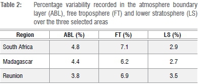
In terms of vertical variation of CO, three principal layers are identified: the atmospheric boundary layer, the free troposphere and the lower stratosphere, representing 1000 hPa to 850 hPa, 850 hPa to 100 hPa, and 100 hPa to 10 hPa, respectively. The relative percentages of deviation with respect to the observed mean values are found in Table 2. Maximum deviation is observed in the free troposphere and minimum deviation in the lower stratosphere. The CO monthly average and its concomitant deviation observed over South Africa and Madagascar, especially in the atmospheric boundary layer, are higher than those observed over Reunion Island. These deviations are most likely a result of local contributions and also possibly due to the lower number of scans achieved by the satellite overpasses over Reunion. The satellite scanning of several regions increases the probability of achieving a variety of daily vertical profiles, which subsequently increase the standard deviation observed for the monthly vertical distributions. On the other hand, the high variability observed over Reunion compared to South Africa and Madagascar in the LS layer is most likely due to the reduced number of observation days recorded per month, most of which are spaced over several days. Hence, the concentrations recorded mainly between the middle and upper troposphere up to stratosphere, may not represent the same structures. As the CO mixing ratio does not change quite as remarkably beyond the tropopause height region, the variability was found to be low, which could be a valid reason for the observed lower deviations.

 

 

Seasonal vertical profile

In order to give an atmospheric dynamic explanation to the observed seasonal vertical profile distributions, seasonal vertical profiles were calculated on 47 pressure levels between 1000 and 10 hPa. The months were grouped into the South African seasons: summer (December to February), autumn (March to May), winter (June to August) and spring (September to November). The profiles and associated standard deviations obtained for each pressure level are presented in the Figure 7 for all the three regions. From Figure 7, we observe that CO values measured between 1000 hPa and 200 hPa are higher than 80 ppb during the spring having a maximum at about 400 hPa over our study location. During winter, summer and autumn, the seasonal average is still below 80 ppb with a maximum located above 300 hPa except over South Africa during summer where the maximum exceeds 80 ppb and is located at around 300 hPa. It is found that the observed quantity from the surface to approximately 600 hPa during winter exceeds that of summer and autumn because the forest fires that usually start in July. It is apparent from the figure that the maximum CO is located around 400 hPa during the spring over both South Africa and the Indian Ocean region. However, during the summer and autumn the CO mixing ratio is observed to be dominant at pressure levels from approximately 350 hPa to 150 hPa primarily over the Indian Ocean region.

 

 

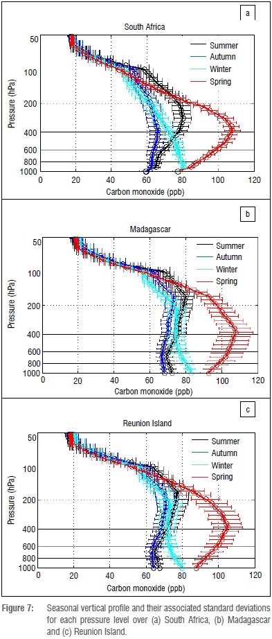
Above 400 hPa, the profiles observed during winter and autumn have the same vertical variation. CO levels observed at 800 hPa over South Africa are generally always higher than the observations at ground level. This is contrary to Madagascar and Reunion Island, where the ground level has a higher CO concentration than the 800 hPa level, especially during winter, summer and autumn. This high quantity observed at 800 hPa over South Africa compared to the other areas is most likely due to various industrial emissions and stable circulation layers, amongst other reasons.

South Africa is located approximately at 30°S of latitude; where the Hadley cell from the tropical region and the Ferrell cell from the middle latitude converge to form a sub-tropical jet-stream. The jet-stream is located at around 300 hPa and extends up to the tropopause region. This tropospheric air current from the west also has a high speed (~25 m/s) and acts as a pathway for moving and transporting air masses and pollutants to the east. A previous study by Stohl et al.²⁶ demonstrated that emission from South America can be advected into the Atlantic to reach southern Africa, thus it can also be transported from South Africa to Australia by crossing the Indian Ocean. The CO transport over the western Indian Ocean region is also governed by the trade winds. Stohl et al.²⁴ has also shown that CO, with a lifetime exceeding 25 days, may reach ~9 km (~300 hPa) over Africa. The effects of trade winds are evident until approximately 6 km altitude (~450 hPa) where there is air mass and pollutants exchange (jet stream-trade wind) in the pressure range from 450 hPa to 300 hPa. This exchange results in homogeneity between the vertical profiles found within the Indian Ocean area (Reunion and Madagascar) and the subtropical zone of South Africa. Thus, because of the jet stream-trade wind exchange and the longer lifetime of CO over Africa, it is also expected that the CO concentrations observed may reach a maximum at approximately 400 hPa over southern Africa and the Indian Ocean during spring.

Deep convection within the ITCZ over the continental region in the southern summer continuously lifts the tropopause upwards by some kilometres and as such deepens the extent of the troposphere. This happens as a result of thunderstorm activity mixing tropospheric air at a moist adiabatic lapse rate, thus pollutants can be transported by vertical convection up to 200 hPa. As a result of this mixing, maximum CO is usually observed at around 200 hPa especially over Madagascar and Reunion Island. This observation also explains why the tropopause layer may, on occasion, move above 200 hPa. This can be clearly seen from 100 hPa level where the seasonal vertical profiles have identical variation. These results confirm that the tropopause is at its lowest level of the atmosphere during the spring and at its highest levels during the others periods. During summer, a maximum CO is observed at around 300 hPa over South Africa and above 200 hPa over Madagascar and Reunion Island. We assume the existence of a dynamic structure that prevents CO convection movements. This dynamic structure is probably located below 200 hPa in the mid-latitudinal region and around 150 hPa in the tropical region, especially during summer, and this may be regarded as the CO tropopause height.

Seasonal distribution of total column CO over the three sites

In this study, the annual cycle of CO distribution was obtained by combining 5 years of TES data, which included 2005, 2006, 2007, 2008 and 2009. The obtained seasonal distribution is plotted in Figure 8. The recorded quantities of CO in January, February and March were lower and are associated with small standard deviations as well. However, the recorded values during this period were higher over Madagascar compared to South Africa and Reunion. The minimum annual CO concentration over Reunion Island and Madagascar occurred during March whilst in May over South Africa, (mainly as a result of the factors discussed in the section on the climatology of CO above). During May, June and July (austral winter), the CO distribution over Reunion Island was similar to that observed over Madagascar. During the same period, the monthly CO values observed over South Africa were below 2.1 ppm. The annual maximum occurred during spring and reached its peak value in September over South Africa (2.8 ± 0.2 ppm) and a month later, in October, over Reunion Island (2.9 ± 0.2 ppm) and Madagascar (3.1 ± 0.2 ppm).

 

 

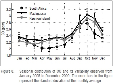
The high CO observed over Madagascar during December, January and February may be caused by emission sources from northern Africa, India and the Middle East, which are transported via western trade winds to the ITCZ (usually located above the Madagascar area during this time). The ITCZ constitutes a convective source and is an effective and significant pollution trapping zone.¹³ From March onwards, the ITCZ migrates to the northern hemisphere after which Madagascar and Reunion Island receive the same climatic conditions as the rest of the study area and thus have the same characteristics which regulate the CO distribution within the mid-latitudes. This is the reason why the monthly observed CO levels over Reunion and Madagascar, especially during April, May, June and July are so similar.

During the austral winter, CO lifetime is typically longer (around a month) within the tropical region.²⁵ This could be a reason why more CO is observed over Madagascar and Reunion Island (tropical zone) during April to July, but is less pronounced over South Africa (mid latitude). However, the CO levels observed over the Indian Ocean region cannot adequately explain the high CO mixing ratio recorded during spring since it generalises over the three study sites and the climatology over South Africa is different from that of the other two sites. As mentioned earlier, the high CO mixing ratio observed during spring is generally associated with increased biomass burning activity over sub-equatorial Africa, Madagascar and southern America.^25,26 Also, the CO transport takes sufficient time to reach the Indian Ocean and could be a reason for the observed high background values of ambient CO during July to August at Cape Point, maximum in September over South Africa and in October over the Indian Ocean. However, a more in-depth investigation on CO-coupled air mass trajectories at a regional and continental scale is needed to validate this statement.

Trend estimates

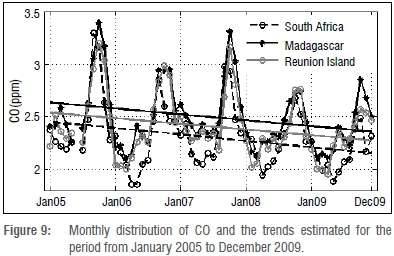
Trend analyses were carried out using the monthly mean values of CO for the 5-year period from 2005 to 2009. The monthly values for the year are represented by integration of the quantities measured over the entire 47 pressure levels. The inter-annual distribution, which is derived from the monthly mean variation, is presented in Figure 9. Positive anomalous were evident in 2005 and 2007 and negative anomalous were observed during the summers of 2006, 2008 and 2009. In the framework of the annual emission budget, higher quantities were observed in 2005 and 2007 while lower quantities were recorded in 2006, 2008 and 2009.

 

 

Two important events were observed during the spring of 2005 and 2007 which contributed significantly to the high quantities observed in those years: (1) the El Nino events and (2) an increase in biomass burning activity. Indeed, the El Nino events that occurred in 2005 and 2007 were associated with positive anomalies of total column CO over the entire globe, except for high latitudes of the two hemispheres.²⁷ In addition, 2005 and 2007 were marked by an increase in biomass burning activity in the southern hemisphere, especially over the South America area, according to Torres et al.²⁸ and Giglio et al.²⁹

As the annual cycle of CO is strongly linked with biomass burning activity in the southern hemisphere,^28,30,31 we assume that the low quantity observed in 2006 was partly due to the reduced biomass burning activity in the South American region. This happened as a result of the tri- national committee action and small farmer initiative which both aimed to reduce biomass activity in 2006.^30,31 A study by Torres et al.²⁸ showed strong negative anomalies of biomass burning activity during 2008 and 2009 in the southern hemisphere. Their inter-annual fire account and aerosol optical absorption distributions were shown to have similar lower peaks upon comparison with our CO inter-annual distribution results (Figure 9) over the same period. In addition, Yongxing²⁷ showed that the reduced CO levels observed in 2006, 2008 and 2009 were partly due to La Nina events which were observed in January and February of 2006, 2008 and 2009. These events are normally associated with heavy rainfalls, which can considerably decrease the amount of pollutants within the atmosphere while reducing the total biomass burning events themselves. Therefore, the observed inter-annual variability in Figure 9 is primarily a result of a mixture of biomass burning and El Nino Southern Oscillation (ENSO) events.

A linear regression was applied on the total column CO data for the three sites under investigation. The results obtained are also plotted in Figure 9. Overall, a negative trend was observed for all three sites. The calculated slopes of the linear trends, quantifying the total column CO decrease, amounted to 5.1 ppb per month, 4.7 ppb per month and 4.5 ppb per month for South Africa, Madagascar and Reunion respectively. Expressed as a percentage, the quantity of CO measured within the 47 pressure levels decreased by 2.1%, 1.8% and 1.7% respectively over South Africa, Madagascar and Reunion.

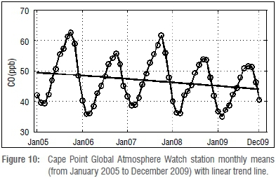
An interesting aspect is that the decreased trend within the CO mixing ratio, observed for our study period (2005-2009), was also reflected within the surface-based measurements of Cape Point (Figure 10). These measurements also show a declining trend of similar magnitude to that observed by the TES/Aura satellite over the three study sites. Figure 10 represents the inter-annual background CO distribution observed at Cape Point (January 2005 to December 2009), derived from mean monthly observations. A linear regression applied on the Cape Point inter-annual distribution, showed that tropospheric CO decreased by a similar negative rate, estimated at 0.1 ppb per month, which corresponds to 2.4% of the average annual mean for this period.

 

 

The concomitant observed decreases in CO mixing ratios observed by TES for the three sites studied is most likely a consequence of activities that drive, or at least can be linked to, the origins of the observed inter-annual CO distribution. These driving processes were discussed earlier in this paper and are: the reduction of biomass burning activity observed in 2006, 2008 and 2009 around South America and the La Nina events with their associated positive rainfall anomalies. The observed decrease in CO is probably also in part due to a reduction in anthropogenic carbon monoxide emissions as suggested by Zeng et al.¹⁶ and/or an increase in global hydroxyl radical (OH),^32,33 but changes within these driving mechanisms need to be verified by further studies. A recent study by Zeng et al.¹⁶ analysed the CO trend over two southern hemisphere sites (Lauder, New Zealand (45°S, 170°E) and Arrival Height, Antarctica (78°S, 167°E )) between 1997 and 2010. They reported a decreasing rate of CO, estimated to be around -0.94 ± 0.47% per year. They further explored the relationship between this negative rate and an overall decline in CO emissions from industrial sources, estimated to be around 26% in the southern hemisphere for the period from 1997 to 2009.

The atmospheric oxidant capacity depends directly on the amount of OH radical available. This very reactive species acts as the tropospheric detergent, by reacting with most of the emitted oxidants, and especially CO.³⁴ Therefore, OH distributions determine the CO lifetime in the atmosphere.²¹ A study by Prinn et al.³³ has shown an increase of the global hydroxyl radical (OH) in the atmosphere, estimated to be around 1.0 ± 0.8% per year from 1979 to 1990. However, more investigations on OH distributions over our study area during the study period are needed in order to validate this statement.

 

Summary and conclusion

In this study, we investigated spatiotemporal distributions of CO over three different adjacent regions, namely South Africa, Madagascar and Reunion using five years (2005-2009) of data obtained from the TES Aura satellite instrument. A preliminary study was conducted to validate TES data through comparison with ground-based CO data recorded at the Cape Point GAW station. A comparison was performed between ground-based measurements uncontaminated by continental air mass and satellite data recorded at 1000 hPa over the Cape Point station and a satisfactory agreement was found between the measurements. The mean bias error observed between the two observations was 6.6% and the regression coefficient was greater than 0.6. Thereafter, data from the TES instrument was used to investigate CO variation and trends on the three selected regions. The following are salient features noted from this study:

• Monthly and seasonal vertical distributions obtained from 47 pressure levels of TES data highlighted the most prominent pressure ranges of pollutants within the free troposphere, being from 400 hPa to below 150 hPa. As a result of CO having a long lifetime within these pressure ranges, a mechanism is in place, which allows for pollutant transport on a regional and global scale, which includes vertical convective movement, the trade winds and the jet-stream.
• The bulk of the CO concentration was observed in the free troposphere, between 850 hPa and 150 hPa. Above 150 hPa, CO mixing ratio decreased linearly reaching a minimum value at approximately 50 hPa. The lowest CO mixing ratio was observed within the stratosphere.
• An investigation into the temporal variation of CO revealed a high concentration of CO during spring, driven primarily by fires and biomass burning activities over Africa and adjacent regions. The peak period was observed to be between July and October. The quantity of CO observed during this period was estimated to be approximately 45% of the annual recorded values. The minimum CO mixing ratio was observed during the southern summer, specifically during May over South Africa and March over the Indian Ocean region.
• Analyses for the inter-annual distribution of CO identified positive anomalies in the spring of 2005 and 2007 and lower quantities of CO during 2006, 2008 and 2009.
• A linear regression applied on inter-annual CO variation exhibited a negative trend in the order of 2.1% over South Africa, 1.8% over Madagascar and 1.7% over Reunion. The observed declining rate of CO in the upper atmosphere was also confirmed with an analysis made on ambient surface CO at the Cape Point GAW station which displayed a tropospheric background CO decline, estimated at approximately 2.4% per year.

From these analyses, we conclude that measurements of CO using TES are in agreement with ground-based measurements. TES can therefore be used for future analyses on the variability of CO in southern tropic and middle latitude regions, or TES measurements could be merged with correlative data to provide a high-quality and reliable long-term CO data set.

 

Acknowledgements

This work is supported by the GDRI ARSAIO (Atmospheric Research in Southern Africa and the Indian Ocean), a French-South African cooperative programme network supported by the French Centre National de la Recherche Scientifique (CNRS) and the South African National Research Foundation (NRF). A.M.T. acknowledges the Indian Ocean Bureau AUF (Agence Universitaire de la Francophonie) and the University of KwaZulu-Natal for travel and hosting invited student exchange on the NRF-CNRS bi-lateral research project (UID 78682). We also thank the TES team and the South Africa Weather Service for providing the CO data used in this work. S.K.S. acknowledges the SANSA Earth Observation for their financial support.

 

Authors' contributions

A.M.T. was the project leader; V.S. was the supervisor of the project and the principal coordinator of the ARSAIO (Atmospheric Research Southern Africa and Indian Ocean) programme; N.M., S.S. and H.B. contributed to data analysis and the review of the manuscript. E.G.B. and C.L. assisted in interpreting the results and writing the paper.

 

References

1. Clerbaux C, George M, Turquety S, Walker KA, Bernath P Barret B, et al. CO measurement from the ACE-FTS satellite instrument: Data analysis and validation using ground-based, airborne and spaceborne observation. Atmos Chem Phys. 2008;8:2569-2594. http://dx.doi.org/10.5194/acp-8-2569-2008        [ Links ]

2. Beer R. TES on the aura mission: Scientific objectives, measurement, and analysis. IEE Trans Geosci Remote Sens. 2006;44:1102-1105. http://dx.doi.org/10.1109/TGRS.2005.863716        [ Links ]

3. Herman R, Kulawik S. Tropospheric Emission Spectrometer (TES), Level 2 (L2) data user's guide version 5. Pasadena, CA:JPL; 2011.         [ Links ]

4. Kopacz M, Daniel JJ, Daven KH, Heald LC, David GS, Qiang Z. Comparison of adjoint and analytical Bayesian inversion method for constraining Asian source of CO, using satellite (MOPITT) measurement of CO columns. J Geophys Res. 2009;114(D04305):1-10.         [ Links ]

5. Luo M, Beer R, Jacob DJ, Logan JA, Rodgers CD. Simulated observation of tropospheric ozone and CO with the TES satellite instrument. J Geophys Res. 2002;107(D15):ACH9 1-10.         [ Links ]

6. Luo M, Rinsland CP, Rodgers CD, Logan JA, Worden H, Kulawik S, et al. Comparison of carbon monoxide measurements by TES and MOPITT: Influence of a priori data instrument characteristics on nadir atmospheric species retrievals. J Geophys Res. 2007;112(D9), 303, 13 pages.         [ Links ]

7. Heald LC, Jacob DJ, Jones DBA, Palmer PI, Logan JA, Streets DG, et al. Comparative inverse analysis of satellite (MOPITT) and aircraft (TRACE-P) observation to estimate Asian source of CO. J Geophys Res. 2004;109(D23), 306, 17 pages.         [ Links ]

8. Richards NAD, Li Q, Bowman KW, Worden JR, Kulawik S, Osterman GB, et al. Assimilation of TES CO into a global CTM: First results. Atmos Chem Phys Discuss. 2006;6:11727-11743. http://dx.doi.org/10.5194/acpd-6-11727-2006        [ Links ]

9. Kopacz M, Jacob DJ, Fisher JA, Logan JA, Zhang L, Megretskaia IA, et al. Global estimation of CO sources with high resolution by adjoint inversion of multiple satellite datasets (MOPITT, AIRS, SCHIAMACHY and TES). Atmos Chem Phys. 2010;10:855-876. http://dx.doi.org/10.5194/acp-10-855-2010        [ Links ]

10. Yurganov LN, Rakitin V Dzhola A, August T, Fokeeva E, George M, et al. Satellite- and ground-based CO total column observations over 2010 Russian fires: Accuracy of top-down estimates based on thermal IR satellite data. Atmos Chem Phys. 2011;11:7925-7942. http://dx.doi.org/10.5194/acp-11-7925-2011        [ Links ]

11. Rajab JM , MatJafr MZ, Lim HS, Abdullahi K. Indonesia forest fires exacerbate carbon monoxide pollution over peninsular Malaysia during July to September 2005. 6th International Conference on Computer Graphics Imaging and Visualisation (ICCGIV09); 2009 Aug 11-14; Tianjin, China. Washington DC: IEEE; 2009. p. 547-552.         [ Links ]

12. Duflot V Dils B, Baray JL, De Mazière M, Attié JL, Vanhaelewyn G, et al. Analysis of the origin of the distribution of CO in the subtropical southern Indian Ocean in 2007. J Geophys Res. 2010;115(D22), 106, 16 pages.         [ Links ]

13. De Laat ATJ, Lelieveld J, Roelofs GJ, Dickerson RR, Lobert JM. Source analysis of carbon monoxide pollution during INDOEX 1999. J Geophys Res. 2001;106:28481-28495. http://dx.doi.org/10.1029/2000JD900769        [ Links ]

14. Khalil KAM, Rasmussen RA. Global decrease in atmosphere carbon monoxide concentration. Nature. 1994;370:639-641. http://dx.doi.org/10.1038/370639a0        [ Links ]

15. Novelli PC, Masarie KA, Tans PP, Lang PM. Recent changes in carbon monoxide. Science. 1994;263:1587-1590. http://dx.doi.org/10.1126/science.263.5153.1587        [ Links ]

16. Zeng G, Wood SW, Morgenstern O, Jones NB, Robinson J, Smale D. Trends and variations in CO, C₂H₆, and HCN in the southern hemisphere point to the declining anthropogenic emissions of CO and C₂H₆. Atmos Chem Phys. 2012;12:7543-7555. http://dx.doi.org/10.5194/acp-12-7543-2012        [ Links ]

17. Hammer S, Mattheier HG, Muller L, Sabasch M, Schimdt M, Schmitt S, et al. A gas chromatography system for high precision quasi-continuous atmospheric measurement of CO₂, CH₄, N₂O, SF₆, CO and H₂ [document on the Internet].         [ Links ] c2008 [cited 2014 Feb 20]. Available from: http://www.iup.uni-heidelberg.de/institut/forschung/groups/kk/GC_Hammer_25_SEP_2008.pdf

18. Scheel HE, Brunke EG, Sladkovic R, Seiler W. In situ CO concentrations at the sites Zugspitze (47°N, 11°E) and Cape Point (34°S, 18°E) in April and October 1994. J Geophys Res. 1998;103(D15):19295-19304. http://dx.doi.org/10.1029/96JD04010        [ Links ]

19. Brunke EG, Labuschagne C, Parker B, Scheel HE, Whittlestone S. Baseline air mass selection at Cape Point, South Africa: Application of ²²²Rn and other filter criteria to CO₂. Atmos Environ. 2004;38(33):5693-5702. http://dx.doi.org/10.1016/j.atmosenv.2004.04.024        [ Links ]

20. Swap R, Annegarn HJ, Suttles TS, King MD, Platnick S, Privette JL, et al. Africa burning: A thematic analysis of the southern African regional science initiative (SAFARI 2000). J Geophys Res. 2003;108(D13):SAF 1-14.         [ Links ]

21. Novelli PC, Masarie KA, Lang PM. Distribution and recent changes of CO in the lower troposphere. J Geophys Res. 1998;103:19015-19033. http://dx.doi.org/10.1029/98JD01366        [ Links ]

22. Wang C, Prinn R. Impact of emissions, chemistry, and climate on atmospheric carbon monoxide: 100-year predictions from a global chemistry-climate model. Chemosphere Global Change Sci. 1999;1(1-3):73-81. http://dx.doi.org/10.1016/S1465-9972(99)00016-1        [ Links ]

23. Brunke EG, Ebinghaus R, Kock HH, Labuschagne C, Slemr F. Emissions of mercury in southern Africa derived from long-term observations at Cape Point, South Africa. Atmos Chem Phys. 2012;12:7465-7474. http://dx.doi.org/10.5194/acp-12-7465-2012        [ Links ]

24. Stohl A, Sabine E, Caroline F, Paul J, Nicole S. On the pathways and timescales of intercontinental air pollution transport. J Geophys Res. 2002;107(D23):ACH6-1-ACH6-17        [ Links ]

25. Duflot V. Quantification et étude du transport des polluants dans la troposphère de l'Océan Indien [Quantification and study of pollutants transport in the stratosphere of the Indian Ocean] [thesis].         [ Links ] Saint Denis: LACy, University of Réunion; 2012. French.

26. Van der Werf GR, Randerson JT, Gilio L, Collatz GJ, Kasibhatla PS, Arellano AF. Inter-annual variability in global biomass burning emission from 1997 to 2004. Atmos Chem Phys. 2006;6:3423-3441. http://dx.doi.org/10.5194/acp-6-3423-2006        [ Links ]

27. Yongxing Z. Mean global and regional distribution of MOPPIT carbon monoxide during 2000-2009 and during ENSO. Atmos Environ. 2010;45:1347-1358.         [ Links ]

28. Torres O, Chen Z, Jethva H, Ahn C, Freitas SR, Bhartia PK. OMI and MODIS observations of the anomalous 2008-2009 southern hemisphere biomass burning seasons. Atmos Chem Phys. 2010;10:3505-3513. http://dx.doi.org/10.5194/acp-10-3505-2010        [ Links ]

29. Giglio L, Randerson JT, Van der Werf GR, Kasibhatla PS, Collatz GJ, Morton DC, et al. Assessing variability and long-term trends in burned area by merging multiple satellite fire products. Biogeosciences. 2010;7:1171-1186. http://dx.doi.org/10.5194/bg-7-1171-2010        [ Links ]

30. Koren I, Remer LA, Longo K. Reversal of trend of biomass burning in the Amazon. Geophys. Res. Lett. 2007;34(L20), 404, 4 pages.         [ Links ]

31. Koren I, Remer LA, Longo K, Brown F Lindsey R. Reply to comment by W. Schroeder et al. on ''Reversal of trend of biomass burning in the Amazon''. Geophys Res Lett. 2009;36(L03), 807. http://dx.doi.org/10.1029/2008gl036063        [ Links ]

32. Prinn RG, Huang J. Comment on "Global OH trend inferred from methylcloroform measurements" by Maarten Krol et al. J Geophys Res. 2001;106:23151-23157. http://dx.doi.org/10.1029/2001JD900040        [ Links ]

33. Prinn RG, Cunnold DP Simmonds F, Alyea R, Boldi A, Crawford P Global average concentration and trend for hydroxyl radicals deduced from ALE/GAGE trichloroethane (methyl chloroform) data for 1978-1990. J Geophys Res. 1992;97:2445-2461. http://dx.doi.org/10.1029/91JD02755        [ Links ]

34. Duncan BN, Logan JA. Model analysis of the factors regulating the trends and variability of CO between 1988 and 1997. Atmos Chem Phys. 2008;8:7389-7404. http://dx.doi.org/10.5194/acp-8-7389-2008        [ Links ]

 

 

Correspondence:
Abdoulwahab Toihir
Laboratoire de l'Atmosphère et des Cyclones UMR
8105, 15 Avenue René Cassin
Université de la Réunion, CS 92003
97744 Saint-Denis, Cedex, Réunion
France
Email: fahardinetoihr@gmail.com

Received: 28 May 2014
Revised: 10 Dec. 2014
Accepted: 25 Apr. 2015