RESEARCH ARTICLE

 

Modelling of extreme minimum rainfall using generalised extreme value distribution for Zimbabwe

 

 

Delson Chikobvu^I; Retius Chifurira^II

^IDepartment of Mathematical Statistics and Actuarial Sciences, University of the Free State, Bloemfontein, South Africa
^IISchool of Mathematics, Statistics and Computer Science, University of KwaZulu-Natal, Durban, South Africa

Correspondence

 

 

---

ABSTRACT

We modelled the mean annual rainfall for data recorded in Zimbabwe from 1901 to 2009. Extreme value theory was used to estimate the probabilities of meteorological droughts. Droughts can be viewed as extreme events which go beyond and/or below normal rainfall occurrences, such as exceptionally low mean annual rainfall. The duality between the distribution of the minima and maxima was exploited and used to fit the generalised extreme value distribution (GEVD) to the data and hence find probabilities of extreme low levels of mean annual rainfall. The augmented Dickey Fuller test confirmed that rainfall data were stationary, while the normal quantile-quantile plot indicated that rainfall data deviated from the normality assumption at both ends of the tails of the distribution. The maximum likelihood estimation method and the Bayesian approach were used to find the parameters of the GEVD. The Kolmogorov-Smirnov and Anderson-Darling goodness-of-fit tests showed that the Weibull class of distributions was a good fit to the minima mean annual rainfall using the maximum likelihood estimation method. The mean return period estimate of a meteorological drought using the threshold value of mean annual rainfall of 473 mm was 8 years. This implies that if in the year there is a meteorological drought then another drought of the same intensity or greater is expected after 8 years. It is expected that the use of Bayesian inference may better quantify the level of uncertainty associated with the GEVD parameter estimates than with the maximum likelihood estimation method. The Markov chain Monte Carlo algorithm for the GEVD was applied to construct the model parameter estimates using the Bayesian approach. These findings are significant because results based on non-informative priors (Bayesian method) and the maximum likelihood method approach are expected to be similar.

Keywords: minima; return level; mean annual rainfall; Bayesian approach; severe meteorological drought

---

 

 

Introduction

Relatively extreme low rainfall attributed to global warming, although rare, is a natural phenomenon that affects people's socio-economic activities worldwide. Extreme droughts occur from time to time in Zimbabwe, and impact negatively on the country's economic performance. The drought of rainfall season year 1991/1992 was one of the worst in the recorded history of Zimbabwe. Its impact was felt even in the insurance industry which received high claims for crop failure.¹ Droughts can be viewed as extreme events outside of the normal rainfall occurrences, such as exceptionally lower amounts of mean annual rainfall.² In Zimbabwe, at least 50% of the gross domestic product is derived from rain-fed agriculture.³ With more low technology indigenous farmers entering commercial agriculture through the accelerated land-reform programme, modelling and prediction of extreme low annual rainfall and the associated probabilities of drought become more relevant.

Developing methods that can give a suitable prediction of meteorological events is always interesting for both meteorologists and statisticians. The use of standard statistical techniques in modelling, forecasting and prediction of extremes in average rainfall and rare events is less prudent because of gross under-estimation.⁴ Extreme value theory is an alternative and superior approach to quantify the stochastic behaviour of a process at unusually large or small levels.⁴ Extreme value theory provides the statistical framework to make inferences about the probability of very rare and extreme events. It is based on the analysis of the maximum (or minimum) value in a selected time period.

Recently there has been growing interest in modelling extreme events, especially in situations in which scientists underestimated the probabilities of extreme events that subsequently occurred and caused catastrophic damage.⁵ Work has been done which provides evidence of the importance of modelling rainfall from different regions of the world: Nadarajah and Choi⁶ used extreme value theory for rainfall data from South Korea; Koutsoyiannis⁷ applied extreme value theory to rainfall data from Europe and the USA; Koutsoyiannis and Baloutsos⁸ applied extreme value theory to Greece's rainfall data; and Crisci et al.⁹ applied extreme value distributions to rainfall data from Italy. The use of extreme value distributions is not restricted to meteorology events; examples appear in energy¹⁰; insurance¹¹; fish management¹² and ecology¹³. There is no work known to us on rainfall extremes in Zimbabwe. In this paper, we provide the first application of extreme value distributions to model minimum annual rainfall in Zimbabwe.

Rainfall in Zimbabwe is associated with the behaviour of the inter-tropical convergence zones whose oscillations are influenced by changing pressure patterns to the north and south of the country.¹⁰ Zimbabwe lies in the Southwest Indian Ocean zone, which is often affected by tropical cyclones. Tropical cyclones are low pressure systems that have well-defined clockwise (in the southern hemisphere) wind circulations which spiral toward the centre where the winds are strongest and rains are heaviest. Cyclones that develop over the western side of the Indian Ocean occasionally affect the rainy season. The amount and intensity of rainfall during a given wet spell is enhanced by the passage of upper westerly wind waves of mid-latitude origin.^14,15

Studies of extreme low rainfall are beneficial to decision-makers in government, non-governmental organisations involved in early warning systems and food security, poverty alleviation and disaster management and risk management. This study will also inform climatologists about the behaviour of extreme low rainfall. Appropriate decisions and plans can be made based on the results of this study to prepare the general public for changes brought on by extremely low rainfall. The objective of this study was to quantify and describe the behaviour of extremely low rainfall in Zimbabwe. In particular, the aim was to model the extreme low rainfall using the generalised extreme value distribution (GEVD) by using the maximum likelihood estimation method and the Bayesian statistics approach. The mean return period - that is, the number of years on average before another drought of equal or greater intensity - was also calculated.

 

Research methodology

Normal distribution

A normal distribution is symmetrical and has a bell-shaped density curve with a single peak. The normal density function, which gives the height of the density at any value x is given by:

where μ is the mean (where the peak of the density occurs) and σ is the standard deviation (which indicates the spread or girth of the bell curve).

Generalised extreme value distribution

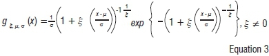
In climatology, meteorology and hydrology, maxima of temperatures, precipitation and river discharges have been recorded for many decades.¹⁶ The extreme value theorem provides a theoretical framework to model the distribution of extreme events and the three-parameter GEVD was recommended for meteorology frequency analysis.¹⁷ The three parameters are: location, scale and shape. The GEVD is a family of continuous probability distributions developed within the extreme value theorem. The GEVD unites the Gumbel, Fréchet and Weibull family of distributions into a single family to allow a continuous range of possible shapes. Based on the extreme value theorem, the GEVD is the limiting distribution of properly normalised maxima of a sequence of independent and identically distributed random variables.¹⁸ Thus, the GEVD is used to model the maxima of a long (finite) sequence of random variables. The unified GEVD for modelling maxima is given by:

where μ, σ and ξ are the location, scale and shape parameters, respectively. The probability density function is sometimes called the Fisher-Tippett distribution and is obtained as the derivative of the distribution function:

The shape parameter ξ is also known as the extreme value index. The parameter ξ^-1is the rate of tail decay of the GEVD. If ξ > 0, G belongs to the heavy-tailed Fréchet class of distributions such as Pareto, Cauchy, student-t and mixture distributions. If ξ < 0, G belongs to the short-tailed with finite lower bounds Weibull class of distributions which includes distributions such as uniform and beta distributions. If ξ = 0 then G belongs to the light-tailed Gumbell class of distributions which includes distributions such as normal, exponential, gamma and log-normal distributions.¹⁹

Modelling minima random variables

The classical GEVD for extremes is based on asymptotic approximations to the sampling behaviour of block maxima. The block maxima size (hourly, daily, weekly, monthly or yearly) varies according to instrument constraints, seasonality and the application at hand. The only possible limiting form of a normalised maximum of a random

sample (when a non-degenerate limit exists) is captured by the GEVD. The data set is partitioned into blocks of equal length and distribution and GEVD is fitted to the set of block maxima. In this study, minima rainfall was modelled using GEVD. In order to model minima random variables we use the duality between the distributions for maxima and minima. If M_N= min{X₁,X₂...,X_N} where X₁,X₂,...,X_Nis a sequence of independent random variables having a common distribution function and Y_i = -X_ifor i = 1,..,N the change of sign means that small values of X_i correspond to large values of Y_i So if M_N= min{X₁,X₂...,X_N} and = max{Y₁,Y₂ ,...,Y_N}, then M_N= -M_N. The minima becomes:

where X_i for i = 1,2,3,...,T represents mean annual rainfall in period i. Extreme maxima theory and methods are then used to model extreme minima.^5,20 Based on the extreme value theorem that derives the GEVD, we can fit a sample of extremes to the GEVD to obtain the parameters that best explain the probability distribution of the extremes.

Parameter estimation

There is a wide variety of methods to estimate the GEV parameters in the independent and identically distributed settings.²¹ The three parameters are estimated by method of moments, maximum likelihood method, method of textiles²² and probability weighted moments or equivalent L-moments.¹⁷ Hosking²³ showed that the probability weighted moments quantile estimators for the GEVD are better than the maximum likelihood method for small samples (n < 50). Madsen et al.²⁴ also showed that method of moments quantile estimators perform well when the sample size is modest. In this study, the maximum likelihood method was exploited because n > 50.

Maximum likelihood method

Under the assumption that X₁,...,X_mare independent random samples

having a GEVD, the log-likelihood for the GEVD parameters when ξ≠ 0 is:

provided that 1 + ξ > 0 for i = 1,...,m.⁵We differentiated the log-likelihood of GEVD to find a set of equations which we solved using numerical optimisation algorithms (see Appendix 1 in the online supplementary material). For computational details, we refer to previous studies.^23,25-27 Because the support of G depends on the unknown parameter values, the usual regularity conditions underlying the asymptotic properties of maximum likelihood estimators are not satisfied. This problem is studied in depth by Stephens²⁸. In the case ξ > -0.5, the usual properties of consistency, asymptotic efficiency and asymptotic normality hold.

Test for stationarity

The augmented Dickey Fuller (ADF) stationarity test is performed on the data to test for stationarity. The null hypothesis of the ADF test is that there is no trend while the alternative hypothesis is that there is a trend in the data.

Goodness of fit

To access the quality of convergence of the GEVD, the Kolmogorov-Smirnov (K-S) and Anderson-Darling goodness-of-fit tests were used. The K-S test, based on the empirical cumulative distribution function, is used to decide if a sample comes from the hypothesised continuous distribution. The K-S test is less sensitive at the tails than at the centre of the distribution. The Anderson-Darling test, which is an improvement of the K-S test, compares the fit of an observed cumulative distribution function to an expected cumulative distribution function; this test gives more weight to the tails of a distribution than does the K-S test.²⁹

Return period or level estimates

We can estimate how often the extreme quantiles occur with a certain return level. The return level is defined as a level that is expected to be equalled or exceeded on average once every interval of time (T) with a probability of p. For the normal distribution we set:

where T is the return period and x_p the return level. By setting the return period and solving the equation (see Appendix 1 in the online supplementary material), the return level, x_pcan be calculated:

which can be re-written as:

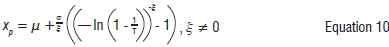
Similarly, for the GEVD we set:

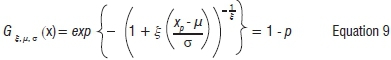
The return level (see Appendix 1 in the online supplementary material) is given by:

Return levels are important for prediction purposes and can be estimated from stationary models. The mean return period is the number of years we expect to wait on average before we observe another drought of equal or greater intensity. If the exceedance probability of observing a drought of a given severity in any given year is p then the mean return period T is such that .

Bayesian analysis of extreme values for GEVD

Inference on the extremes of environmental processes is important to meteorologists, civil engineers, agriculturalists and statisticians. Naturally, data at extreme levels are scarce. Bayesian inference allows any additional information about the processes to be incorporated as prior information. The basic theory of Bayesian analysis of extreme values is well documented (see Coles⁵, Coles and Tawn³⁰ and Gamerman³¹ for more information). The Markov chain Monte Carlo techniques are applied in this paper to give Bayesian analyses of the annual minima rainfall data for Zimbabwe. [The annual maximum rainfall data are given in Appendix 2 of the online supplementary material.] Markov chain Monte Carlo techniques provide a way of simulating from complex distributions by simulating from Markov chains, which have the target distributions as their stationary distributions.³² In this paper, the prior is constructed by assuming there is no information available about the process (rainfall) apart from the data. The annual rainfall data have a GEVD, i.e. X_i~GEVD(µ, σ, ξ) and the parameters μ, σ and ξ are treated as random variables for which we specify prior distributions. For specification of the prior, the parameterisation = log σ is easier to work with because σ is constrained to be positive. The specification of priors enables us to supplement the information provided by the data. The prior density is:

where each marginal prior is normally distributed with large variances. The variances are chosen to be large enough to make the distributions almost flat, corresponding to prior ignorance. The joint posterior density is the product of the prior and the likelihood and is given as:

is the likelihood with σ replaced by . The Gibbs sampler is used to simulate from each of the full conditionals. The posterior is of the form:

so the full conditionals are of the form:

For details of the Markov chain Monte Carlo algorithm refer to R package (evdbayes version1.1-1).

 

Results

Description of data

The analysis was based on the historical mean annual rainfall data recorded from all 62 weather stations in Zimbabwe, dating from as far back as year 1901 to year 2009. A mean annual rainfall figure for the country was calculated. The mean data were obtained from the Zimbabwe Department of Meteorological Services. From Figure 1, it seems reasonable to assume that the pattern variation has stayed stationary over the observation period, and we can model the rainfall data as independent observations from the GEVD. In fitting a 109-year data set to a GEVD, a block size had to be chosen so that individual block minima had a common distribution; yearly blocks were therefore used in this study. Figure 1 shows the graph of x_i , i = 1,...,n the annual rainfall for Zimbabwe.

 

 

The duality principle between the distribution of minima and maxima to fit the distribution of minimal rainfall for Zimbabwe was employed. Maximum likelihood estimates of parameters were estimated (see Appendix 1 in the online supplementary material). Figure 2 shows the graph of -x_i annual rainfall for Zimbabwe.

 

 

Unit root test for stationarity

The augmented Dickey Fuller (ADF) test was used to check for stationarity of -x_i annual rainfall for Zimbabwe. Table 1 shows the results of the ADF test.

 

 

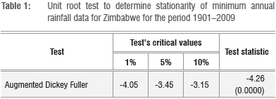
The p-values of the ADF test statistics are significant; we therefore reject the null hypothesis of no stationary at 1%, 5% and 10% levels of significance and conclude that the rainfall data are stationary. The ADF test also indicates that the data do not follow any trend. Therefore, we can determine the return levels of minima annual rainfall.

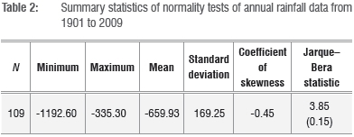
Descriptive statistics

Table 2 shows the descriptive statistics - specifically the coefficient of skewness and Jarque-Bera normality test - of the 109 years of annual rainfall data. The coefficient of skewness of minima annual rainfall (-x) is negative. This observation suggests that the rainfall data fit a distribution which is relatively long left tailed.

 

 

Fitting distributions to minimum mean annual rainfall Normal distribution

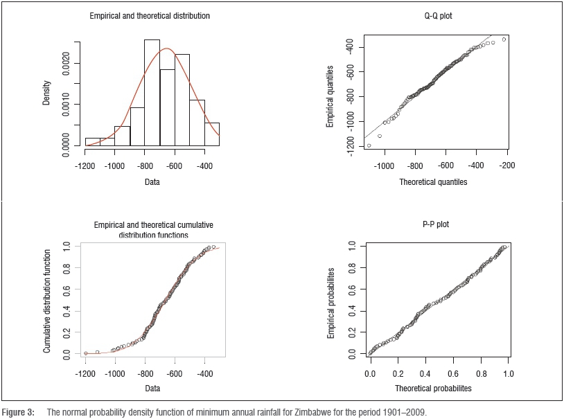
Figure 3 shows the normal probability density function of minima mean annual rainfall data from 1901 to 2009.

The parameter estimates and their corresponding standard errors in brackets are:

= -659.9312 (16.13623)

= 168.4675 (11.41010)

Figure 3 shows the minima mean annual rainfall data normal quantile-quantile (Q-Q) plot of minima annual rainfall for Zimbabwe. The normal Q-Q plot of minima annual rainfall shows deviation from a normal distribution at both lower and upper tails of the data. However, based on the p value of the Jarque-Bera test, we fail to reject the null hypothesis of normality. The question is: If annual rainfall is normally distributed, then how do we account for extremely low rainfall (severe droughts) or extremely high rainfall (severe floods) events that have been recorded? The normal distribution approximates these events as negligible or close to zero. If the distribution of minima annual rainfall is heavy-tailed or skewed, the normal distribution may be misleading. Thus, the normal distribution is not a good fit for these rainfall data. The further one gets into the tails of the distribution, the rarer the event, but the event will be catastrophic if it happens. It is important to fit a distribution that is able to capture the probability of extreme minimum annual rainfall.

Generalised extreme value distribution

Figure 4 shows the diagnostic plots for the goodness of fit of the minima annual rainfall for Zimbabwe from 1901 to 2009.

Table 3 shows the maximum likelihood estimates of the GEVD model with their corresponding standard errors in brackets.

 

 

These results show that the data can be modelled using a Weibull class of distribution because ξ<0 (bounded tail). Combining estimates and standard errors, the 95% confidence intervals for ξ, σ and μ are [-0.5561; -0.3259], [154.8222; 203.7196] and [-744.4090; -670.9278], respectively. ξ is significantly different from zero because zero is not contained in the interval.

Model diagnostic

It is important to confirm that the data adequately fit the GEVD. Figure 3 shows the Q-Q plot and the P-P plot of the data. The quantiles of minima rainfall regressed against the quantiles of GEVD shows a straight line. This finding suggests that the data do not deviate from the assumption that they follow a GEVD. Table 4 shows the K-S and Anderson-Darling statistics.

 

 

The Anderson-Darling statistic is less than its 5% critical value and the K-S statistic test leads to a decision of non-rejection of the null hypothesis. We conclude that the minimum annual rainfall for Zimbabwe follows the specified GEVD.

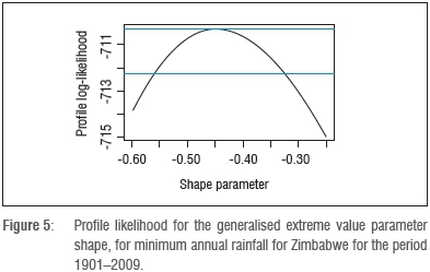
The maximum likelihood estimate for ξ is negative, corresponding to a bounded distribution, in which the 95% confidence interval does not contain zero. Greater accuracy of the confidence interval is achieved by the use of the profile likelihood. Figure 5 shows the profile likelihood of the generalised extreme value parameter ξ, from which a 95% confidence interval for ξ is obtained as approximately [-0.55; -0.45], which is almost the same as the calculated 95% confidence interval.

 

 

Return level estimate

The return levels or periods are estimated using the GEVD. Rainfall less than 473 mm per annum is categorised by the Department of Meteorological Services in Zimbabwe as a meteorological drought. Table 5 shows the return level estimates at selected return intervals T using the GEVD. Mean annual rainfall is expected to be below the drought threshold value of 473 mm in a return period of T=8 years.

 

 

The minimum mean annual rainfall for Zimbabwe was 335.3 mm, recorded in the 1991/1992 rainfall season. This is the worst drought in the recorded history of the country. The return level estimate of 335.2 mm is associated with a mean return period of about 90 years, that is, we expect a drought of similar or worse magnitude in 90 years.

Bayesian analysis of minima annual rainfall data

The Markov chain Monte Carlo method was applied to the annual minimum rainfall data. The GEVD scale parameter was re-parameterised as = log σ to retain the positivity of this parameter. The prior density was chosen to be

for the three parameters of the GEVD, where, for example, N(0,400000) denotes a Gaussian distribution with mean 0 and variance 400 000. These are independent normal priors with large variances. The variances were chosen to be large enough to make the distributions almost flat, corresponding to prior ignorance. In this paper, 30 000 iterations of the algorithm were carried out. Figure 6 shows the Markov chain Monte Carlo trace plots.

 

 

To check that the chains had converged to the correct place, different starting points were used. All the chains converged. The estimated posterior densities for the GEVD parameters for Zimbabwe are given in Figure 7.

 

 

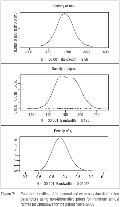
The posterior means and standard deviations for the GEVD parameters are given in Table 6. Using non-informative priors, which are almost flat and add very little information to the likelihood, the posterior means are close to the maximum likelihood estimates of the GEVD parameters given in Table 3. The frequentist properties are preserved by using noninformative priors in the Bayesian statistics approach.

 

 

Conclusion

We modelled extreme minimum annual rainfall in Zimbabwe using the GEVD. Exploring the duality of maxima and minima, annual rainfall data from 1901 to 2009 were fitted to the GEVD. The maximum likelihood estimation method was used to obtain the estimates of the parameters. Model diagnostics, which included the Q-Q plot and the K-S and Anderson-Darling tests, showed that the minimum annual rainfall follows a Weibull class of distribution. The ADF test showed that the minima annual rainfall data were stationary and had no trend. Return level estimates, which are the return levels expected to be exceeded in a certain period, were calculated for Zimbabwe.

The 1992 record drought is likely to return in a mean return period of T = 90 years. The Department of Meteorological Services in Zimbabwe categorises a year with mean annual rainfall below 473 mm as a meteorological drought year. The mean annual rainfall is expected to be less than the drought threshold value of 473 mm in a mean return period of T = 8 years.

The GEVD parameter estimates using the Bayesian approach were close to the maximum likelihood estimates with smaller standard deviations. Using non-informative priors, the frequentist properties of the model are preserved. Using classical statistics is therefore akin to using Bayesian statistics with non-informative priors. Expert opinion, when available in future, can be used to further improve the model. An area of further research is modelling and predicting minimum annual rainfall in Zimbabwe using the Bayesian approach using informative priors. The use of expert priors may improve the precision of the parameters over the maximum likelihood estimates.

 

Authors' contributions

R.C. performed the data analysis and wrote the paper; D.C. supervised R.C., came up with the concept of statistics of extremes to the problem and introduced it to R.C. together with the preliminary analysis and draft on outcomes, provided guidance, and proofread and corrected the paper.

 

References

1. Makarau A, Jury MR. Predictability of Zimbabwe summer rainfall. Int J Climatol. 1997;17:1421-1432. http://dx.doi.org/10.1002/(SICI)1097-0088(19971115)17:13<1421::AID-JOC202>3.0.CO;2-Z        [ Links ]

2. Panu US, Sharma TC. Challenges in drought research: Some perspectives and future directions. Hydro Sci J. 2002;47(S):S19-S30.         [ Links ]

3. Jury MR. Regional tele-connection pattern associated with summer rainfall over South Africa, Namibia and Zimbabwe. Int J Climatol. 1996;16:135-153. http://dx.doi.org/10.1002/(SICI)1097-0088(199602)16:2<135::AID-JOC4>3.0.CO;2-7        [ Links ]

4. Hasan HB, Ahmad NF, Suraiya BK. Modeling of extreme temperature using generalized extreme value (GEV) distribution: A case study of Penang. In: Ao Si, Gelman L, Hukins DWL, Hunter A, Korsunsky AM, editors. Proceedings of the World Congress on Engineering volume 1; 2012 July 4-6; London, UK. Hong Kong: Newswood Limited; 2012. p. 1-6.         [ Links ]

5. Coles S. An introduction to statistical modeling of extreme values. London: Springer; 2001. http://dx.doi.org/10.1007/978-1-4471-3675-0        [ Links ]

6. Nadarajah S, Choi D. Maximum daily rainfall in South Korea. J Earth Sys Sci. 2007;116(4):311-320. http://dx.doi.org/10.1007/s12040-007-0028-0        [ Links ]

7. Koutsoyiannis D. Statistics of extremes and estimation of extreme rainfall: 11 Empirical investigations of long rainfall records. Hydrol Sci J. 2004;49(4):591- 610. http://dx.doi.org/10.1623/hysj.49.4.591.54424        [ Links ]

8. Koutsoyiannis D, Baloutsos G. Analysis of a long record of annual maximum rainfall in Athens, Greece and design rainfall inferences. Nat Hazards. 2000;22:29-48. http://dx.doi.org/10.1023/A:1008001312219        [ Links ]

9. Crisci A, Gozzini B, Meneguzzo F, Pagliara S, Maracchi G. Extreme rainfall in a changing climate: Regional analysis and hydrological implications in Tuscany. Hydrol Process. 2002;6:1261-1274. http://dx.doi.org/10.1002/hyp.1061        [ Links ]

10. Chikobvu D, Sigauke C. Modeling influence of temperature on daily peak electricity demand in South Africa. J Energy South Afr. 2013;24(4):63-70.         [ Links ]

11. Smith RL, Goodman DL. Bayesian risk analysis. Technical report. Chapel Hill, NC: Department of Statistics, University of North Carolina; 2000.         [ Links ]

12. Hilborn R, Mangel M. The ecological detective: Confronting models with data. Monographs on population biology. Princeton, NJ: Princeton University Press; 1997.         [ Links ]

13. Ludwig D. Uncertainty and the assessment of extinction probabilities. Ecol Appl. 1996;6(4):1067-1076. http://dx.doi.org/10.2307/2269591        [ Links ]

14. Buckle C. Weather and climate in Africa. Harlow: Longman; 1996.         [ Links ]

15. Smith SV. Studies of the effects of cold fronts during the rainy season in Zimbabwe. Weather. 1985;(40):198-203. http://dx.doi.org/10.1002/j.1477-8696.1985.tb06869.x        [ Links ]

16. Hosking JRM, Wallis J. Parameter and quantile estimation for the generalized Pareto distribution. Technometrics. 1987;29:339-349. http://dx.doi.org/10.1080/00401706.1987.10488243        [ Links ]

17. Bunya PK, Jain S, Ohjha C, Agarwal A. Simple parameter estimation technique for three-parameter generalized extreme value distribution. J Hydrol Eng. 2007;12(6):682-689. http://dx.doi.org/10.1061/(ASCE)1084-0699(2007)12:6(682)        [ Links ]

18. Beirlant J, Goegebeur Y Segers J, Teugels J. Statistics of extremes: Theory and applications. Chichester: John Wiley & Sons; 2004. http://dx.doi.org/10.1002/0470012382        [ Links ]

19. Bali TG. The generalized extreme value distribution. Econ Lett. 2003;79:423-427. http://dx.doi.org/10.1016/S0165-1765(03)00035-1        [ Links ]

20. Hosking JRM. Testing whether the shape parameter is zero in the generalized extreme value distribution. Biometrika. 1984;71:367-374.         [ Links ]

21. Diebolt L, Guillou A, Rached I. Application of the distribution of excesses through a generalized probability-weighted moments method. J Stat Plan Infer. 2007;137:841-857. http://dx.doi.org/10.1016/j.jspi.2006.06.012        [ Links ]

22. National Environmental Research Council (NERC). Flood studies report. Wallingford: Institute of Hydrology; 1975.         [ Links ]

23. Hosking JRM. Algorithm AS 215: Maximum likelihood estimation of the parameters of the generalized extreme value distribution. Appl Stat. 1985;34:301-310. http://dx.doi.org/10.2307/2347483        [ Links ]

24. Madsen H, Pearson CP Rosbjerg D. Comparison of annual maximum series and partial duration series methods for modelling extreme hydrological events II: Regional modelling. Water Resour Res. 1997;17:1421-1432.         [ Links ]

25. Prescott P Walden AT. Maximum likelihood estimation of the parameters of the generalized extreme value distribution. Biometrika. 1980;67:723-724. http://dx.doi.org/10.1093/biomet/67.3.723        [ Links ]

26. Prescott P, Walden AT. Maximum likelihood estimation of the parameters of the three-parameter generalized extreme value distribution from censored samples. J Stat Comput Sim. 1983;16:241-250. http://dx.doi.org/10.1080/00949658308810625        [ Links ]

27. Macleod AJ. AS R76 - A remark on the algorithm AS 215: Maximum likelihood estimation of the parameters of the generalized extreme value distribution. Appl Stat. 1989;38:198-199. http://dx.doi.org/10.2307/2347695        [ Links ]

28. Smith RL. Maximum likelihood estimation in a class of non-regular cases. Biometrika. 1985;72:67-90. http://dx.doi.org/10.1093/biomet/72.1.67        [ Links ]

29. Stephens MA. EDF statistics for goodness of fit and some comparisons. J Amer Stat Assoc. 1974;69:730-737. http://dx.doi.org/10.1080/01621459.1974.10480196        [ Links ]

30. Coles S, Tawn J. Bayesian modelling of extreme surges on the UK east coast. Philos T Roy Soc A. 2005;363:1387-1406. http://dx.doi.org/10.1098/rsta.2005.1574        [ Links ]

31. Gamerman D. Markov chain Monte Carlo: Stochastic Bayesian inference. London: Chapman and Hall; 1997.         [ Links ]

 

 

Correspondence:
Delson Chikobvu
Department of Mathematical
Statistics and Actuarial Sciences
University of the Free State
PO Box 339, Bloemfontein 9300
South Africa
Email: chikobvu@ufs.ac.za

Received: 06 Aug. 2014
Revised: 04 Nov. 2014
Accepted: 01 Feb. 2015

 

 

Note: This article is supplemented with online only material.