RESEARCH ARTICLE

 

Digital terrain model height estimation using support vector machine regression

 

 

Onuwa Okwuashi^I; Christopher Ndehedehe^II

^IDepartment of Geoinformatics and Surveying, University of Uyo, Uyo, Nigeria
^IIDepartment of Spatial Science, Curtin University, Perth, Australia

Correspondence

 

 

---

ABSTRACT

Digital terrain model interpolation is intrinsically a surface fitting problem, in which unknown heights H are estimated from known X-Y coordinates. Notable methods of digital terrain model interpolation include inverse distance to power, local polynomial, minimum curvature, modified Shepard's method, nearest neighbour and polynomial regression. We investigated the support vector machine regression (SVMR) as a new alternative method to these models. SVMR is a contemporary machine learning algorithm that has been applied to several real-world problems aside from digital terrain modelling. The SVMR results were compared with those from notable parametric (the nearest neighbour) and non-parametric (the artificial neural network) techniques. Four categories of error analysis were used to assess the accuracy of the modelling: minimum error, maximum error, means error and standard error. The results indicate that SVMR furnished the lowest error, followed by the artificial neural network model. The SVMR also produced the smoothest surface followed by the artificial neural network model. The high accuracy furnished by SVMR in this experiment attests that SVMR is a promising model for digital terrain model interpolation.

Keywords: height estimation; artificial neural network; nearest neighbour; algorithm; machine learning

---

 

 

Introduction

Engineers and other related scientists are often charged with the responsibility of producing digital maps that represent the three-dimensional visualisation of the earth's surface. These maps usually serve as auxiliary data for engineering designs of roads, bridges, drainage systems and general landscaping. These digital three-dimensional maps are referred to generically as digital terrain models (DTMs). A DTM is referred to as a 'form of computer surface modelling which deals with the specific problems of numerically representing the surface of the earth'¹.

A DTM is created by using one of two methods: triangulation or gridding. In a gridding method, the corners of regular rectangles or squares are calculated from the scattered control points. In triangulation, triangles are created based on the scattered control points. These triangles do not intersect each other and represent the terrain surface as a linear or non-linear function. In both methods, the heights of grid points and triangular points with unknown heights in the modelled area are estimated by interpolation using their control points.² Notable methods of DTM interpolation include inverse distance to power, local polynomial, minimum curvature, modified Shepard's method, polynomial regression, radial basis function, Kriging and nearest neighbour.^3,4

The aim of this study was to investigate the support vector machine regression (SVMR) model,^5-7 as a new method of DTM interpolation. The goal of the SVMR model is to construct a hyperplane that lies close to as many data points as possible, by choosing a hyperplane that has a small norm that simultaneously minimises the sum of the distances from the data points to the hyperplane. SVMR attempts to minimise the generalisation error bound so as to achieve generalised performance, instead of minimising the observed training error. The idea of SVMR is based on the computation of a linear regression function in a high-dimensional feature space in which the input data are mapped via a non-linear function.⁷ In this experiment, the SVMR results were compared with those from a notable parametric technique (nearest neighbour, NN) and a notable non-parametric technique (artificial neural network, ANN).

 

Support vector machine regression algorithm

For the linear case, given the set of data,

with a linear function

f(x) = (w^.x)+b,⁸ Equation 1

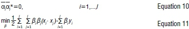
hence the regression function is given by the minimum of the functional

where C is a pre-specified penalty value, and ξ, ξ* are slack variables representing upper and lower constraints, respectively.⁹ Using an ε-insensitive loss function

the solution is given by:

with constraints

The Karush-Kunn-Tucker conditions that are satisfied by the solution are:

with constraints

and the regression function is given by Equation 1, where:

The non-linear SVMR solution using an ε-sensitive function is given by:

with constraints

Solving Equation 16, with constraints Equations 17-19, determines the Lagrange multipliers α_i, α_i* and the regression function is given by:

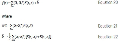
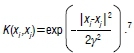
The kernel K(x_i, x_i)can be any of the following common kernel functions: the linear kernel χ-χ, polynomial kernel (x.x+1)^d and radial basis function kernel

 

Methodology

The eastings (E), northings (N) and orthometric heights (H) of 601 points were sampled from a 3.068-ha portion located in southern Nigeria (Figure 1). The sampled area was bounded by UTM coordinates 381810E-382060E and 559700N-559980N (Figure 2). Out of the 601 sampled points, 200 points were selected for training the SVMR algorithm.

 

 

 

 

The experiment was done in MATLAB. The training data contained E, N and H values. E and N were the explanatory variables while H was the target variable. The test data contained just E and N in order to predict the values of H. The SVMR model was trained with known E, N and H values in order to estimate H values of points not used as training data.

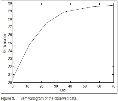
The stratified random sampling was used to select the training data. The spatial dependency of the observed data was examined by plotting its semivariances against the lag distance to produce a semivariogram (Figure 3). The calculated nugget was 0.6. The range was 70, while the sill was 29.6. Beyond the range value the data are spatially independent, whereas the data within the range area are spatially dependent. The nugget value of 0.6 indicated that the error in observation was minimal. The sill value of 29.6 indicated the maximum value of the semivariance that corresponded to the range value.

 

 

The 200 points selected for training and testing were split into classes of 10 (Figure 4). The box plot in Figure 4 shows the statistical distribution of the data. The inner line of the box indicates the median of the data. The top of the upper tail indicates the highest value of the data, while the bottom of the lower tail indicates the lowest value of the data. The experiment was implemented with an optimal ε-sensitive function value ε=0.1. The polynomial, radial basis function and the linear kernels were investigated to select the best kernel function for the experiment, through the method of cross-validation.

 

 

The selection of the optimum kernel parameters' values of degree d, gamma and penalty value C was done using the k-fold cross-validation process where k=10.¹¹ In each experiment, nine data sets (k-1 data sets) were put together to train the SVMR while the remaining one data set was held to test the accuracy of the experiment. The experiment was repeated in 10 folds until all 10 data sets were used for both training and testing (Figure 5).

 

 

 

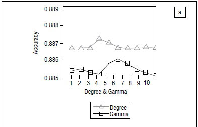
The cross-validation result from Figure 5a shows the accuracy for degree and gamma using values 1 to 10. The value of 4 was found to be the value for degree with the highest accuracy, while 6 was found to be the highest value of gamma with the highest accuracy. From Figure 5b, the values of C with the highest accuracy were 60, 100 and 80 for polynomial, radial basis function and linear kernels, respectively. The polynomial kernel yielded the highest accuracy, and the best value of d was 4 (Figure 5).

 

Results

The resulting DTM and contour plots from interpolation using SVMR are depicted in Figure 6. After interpolation of the heights of the unsampled points using SVMR, the same was implemented with the ANN and NN models.

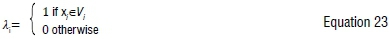
The NN technique predicts the value of an attribute at an unsampled point based on the value of the nearest sample by drawing perpendicular bisectors between sampled points (n), thereby forming polygons (V_i, j=1,2,...,n).⁴ One polygon is produced per sample and the sample is located in the centre of the polygon, such that in each polygon all points are nearer to its enclosed sample point than to other sample points.^12-14 The estimations of the attribute at unsampled points within polygon V_i are the measured value at the nearest single sampled data point x_i, that is The weights are:

All points within each polygon are assigned the same value.^12,14 The NN DTM and contour plots are presented in Figure 7.

The ANN was programmed using multilayer perceptron with a sigmoidal hidden-layer transfer function and linear output neurons. The multilayer perceptron neural network was trained with a back-propagation algorithm, using a two-layer feed-forward neural network. The network had an input layer, an output layer and one or two hidden layers; however, there is no limit to the number of hidden layers.¹⁵ Basically a signal from neuron i of the first input layer of a cell χ at time t received by a neuron j of the hidden layer can be expressed as:

where S'_/ (x,t) denotes the site attributes given by variable (neuron) /; W_ij is the weight of the input from neuron i to neuron j; net_j(x,t) is the signal received for neuron j of cell x at time t.¹⁵ Based on the method of cross-validation, the random seed number was set and the required number of neurons in the hidden layer was set between 1 and 50. The ANN was initialised with initial weights; hence different results were obtained every time the ANN model was run. To ensure the results remained the same at every run of the neural network the random seed number was kept constant. The random seed number is an arbitrary constant chosen by trial and error.

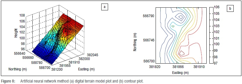
After the random seed number had been set, the number of hidden neurons was the single parameter that was adjusted to obtain simulation results of the ANN. The training of the neural network was done by simply adjusting the number of neurons in the hidden layer in order to minimise the training error. The training error is the discrepancy between the predicted and the actual value. The adjustment of the number of neurons was sustained until the training error fell below a pre-determined threshold.^16-19 The ANN DTM and contour plots are presented in Figure 8.

In Figure 9, the sampled heights were plotted against the 200 points used for the validation of the models. The discrepancies between the observed points and the predicted points using SVMR, ANN and NN are depicted in Figure 9. The plots in Figure 9 show that SVMR yielded the best fit, followed by ANN.

 

 

The experimental errors were calculated by comparing the estimated values using these models with their actual values from the sample. Out of the 601 sampled points, 200 points were selected for training while 50 points were used to test the accuracy of the modelling. The final result was selected from several results obtained by repeating the process, and by re-selecting the training and test data (Figure 10).

 

 

The box plot in Figure 10a shows the statistical error distribution of the data. The inner lines of the box indicate the median of the data. The top of the upper tail indicates the highest value of the data and the bottom of the lower tail indicates the lowest value of the data. From Figure 10a, the calculated minimum error was -1.39, the maximum error was 2.05 and the mean error was -0.07, using the SVMR model. For the ANN model, the calculated minimum error was -1.44, the maximum error was 2.08 and the mean error was -0.09. For the NN model, the calculated minimum error was -2.97, the maximum error was 3.86 and the mean error was 0.35. From Figure 10b, the calculated standard errors for SVMR, ANN and NN were 0.60, 0.65 and 0.81, respectively.

 

Conclusion

The SVMR results were compared with those of the NN and ANN techniques. The NN and ANN are common parametric and non-parametric models, respectively, that have been used in previous studies.³ From Figure 10, we can see that SVMR produced the best results of all the models, followed by the ANN model. The results from the NN model were the least accurate. SVMR also produced the smoothest surface, followed by ANN, while NN produced the roughest surface (Figures 6-8). Even though the SVMR is not a common method of DTM interpolation, our results show that it is a robust technique and can be considered for spatial surface interpolation. However, the differences between the SVMR and ANN results are not significant; more examples are required for the generalisation to be valid.

 

Authors' contributions

O.O. was the project leader, coordinated the research and collected the field data in Nigeria. C.N. performed the laboratory analysis of the field data in Australia.

 

References

1. Heesom D, Mahdjobi L. Effect of grid resolution and terrain characteristics on data from DTM. J Comput Civil Eng. 2001;15(2):137-143. http://dx.doi.org/10.1061/(ASCE)0887-3801(2001)15:2(137)        [ Links ]

2. Yanalak M. Effect of gridding gethod on digital terrain model profile data based on scattered data. J Comput Civil Eng. 2003;1(58):58-67. http://dx.doi.org/10.1061/(ASCE)0887-3801(2003)17:1(58)        [ Links ]

3. Karaborka H, Baykanb OK, Altuntasa C, Yildza F. Estimation of unknown height with artificial neural network on digital terrain model. Vol. XXXVII, Part B3b. Beijing: The International Archives of the Photogrammetry, Remote Sensing and Spatial Information Sciences; 2008.         [ Links ]

4. Li J, Heap AD. A review of spatial interpolation methods for environmental scientists. Geoscience Australia Record. 2008/23. Canberra: Geoscience Australia; 2008. Available from: http://www.ga.gov.au/webtemp/image_cache/GA12526.pdf        [ Links ]

5. Vapnik V. Statistical learning theory. Berlin: Springer; 1998.         [ Links ]

6. Smola AJ, Scholkopf B. A tutorial on support vector regression. NeuroCOLT2 technical report NC2-TR-1998-030 [document on the Internet].         [ Links ] c1998 [cited 2015 Aug 31]. Available from: http://www.svms.org/regression/SmSc98.pdf

7. Gunn S. Support vector machines for classification and regression. ISIS technical report. Southamption: University of Southampton; 1998.         [ Links ]

8. Basak D, Pal S, Patranabis DC. Support vector regression. Neural Inform Process Lett Rev. 2007;11:203-224.         [ Links ]

9. Drucker H, Burges CJC, Kaufman L, Smola A, Vapnik V Support vector regression machines. In: Mozer M, Jordan M, Petsche T editors. Advances in neural information processing systems 9. Cambridge, MA: MIT Press; 1997. p. 155-161.         [ Links ]

10. VapnikV Golowich S, Smola A. Support vector method for function approximation, regression estimation and signal processing. In: Mozer M, Jordan M, Petsche T, editors. Advances in neural information processing systems 9. Cambridge, MA: MIT Press; 1997. p. 281-287.         [ Links ]

11. Bhardwaj N, Langlois R, Zhao G, Lu H. Kernel-based machine learning protocol for predicting DNA-binding proteins. Nucleic Acids Res. 2005;33:6486-6493. http://dx.doi.org/10.1093/nar/gki949        [ Links ]

12. Ripley BD. Spatial statistics. New York: John Wiley & Sons; 1981.         [ Links ]

13. Isaaks EH, Srivastava RM. Applied geostatistics. New York: Oxford University Press; 1989.         [ Links ]

14. Webster R, Oliver MA. Sample adequately to estimate variograms of soil properties. J Soil Sci. 1992;43:177-192. http//dx.doi.org/10.1111/j.1365-2389.1992.tb00128.x        [ Links ]

15. Almeida CM, Gleriani JM, Castejon EF, Soares-Filho BS. Using neural networks and cellular automata for modelling intra-urban land-use dynamics. Int J Geogr Inform Sci. 2008;22(9):943-963. http://dx.doi.org/10.1080/13658810701731168        [ Links ]

16. Rumelhart DE, Hinton GE, Williams RJ. Learning internal representations by error propagation. In: Rumelhart DE, McClelland JL, editors. Parallel distributed processing: Explorations in the microstructure of cognition. Cambridge, MA: MIT Press; 1986. p. 318-362.         [ Links ]

17. Anderson JA. An introduction to neural networks. Cambridge, MA: MIT Press; 1995.         [ Links ]

18. Chauvin Y Rumelhart DE, editors. Backpropagation: Theory, architectures and applications. Hillsdale, NJ: Erlbaum; 1995.         [ Links ]

19. Wang F. The use of artificial neural networks in geographical information systems for agricultural land suitability assessment. Environ Planning A. 1994;26:265-284. http://dx.doi.org/10.1068/a260265        [ Links ]

 

 

Correspondence:
Onuwa Okwuashi
Department of Geoinformatics
and Surveying, University of
Uyo, PMB 1017, Uyo, Aks
Nigeria
Email: onuwaokwuashi@gmail.com

Received: 03 May 2014
Revised: 01 Nov. 2014
Accepted: 03 Feb. 2015