RESEARCH ARTICLE

 

Predictive modelling of wetland occurrence in KwaZulu-Natal, South Africa

 

 

Jens Hiestermann^I; Nick Rivers-Moore^II

^IGeoTerraImage, Pretoria, South Africa
^IICentre for Water Resources Research, University of KwaZulu-Natal, Pietermaritzburg, South Africa

Correspondence

 

 

---

ABSTRACT

The global trend of transformation and loss of wetlands through conversion to other land uses has deleterious effects on surrounding ecosystems, and there is a resultant increasing need for the conservation and preservation of wetlands. Improved mapping of wetland locations is critical to achieving objective regional conservation goals, which depends on accurate spatial knowledge. Current approaches to mapping wetlands through the classification of satellite imagery typically under-represents actual wetland area; the importance of ancillary data in improving accuracy in mapping wetlands is therefore recognised. In this study, we compared two approaches - Bayesian networks and logistic regression - to predict the likelihood of wetland occurrence in KwaZulu-Natal, South Africa. Both approaches were developed using the same data set of environmental surrogate predictors. We compared and verified model outputs using an independent test data set, with analyses including receiver operating characteristic curves and area under the curve (AUC). Both models performed similarly (AUC>0.84), indicating the suitability of a likelihood approach for ancillary data for wetland mapping. Results indicated that high wetland probability areas in the final model outputs correlated well with known wetland systems and wetland-rich areas in KwaZulu-Natal. We conclude that predictive models have the potential to improve the accuracy of wetland mapping in South Africa by serving as valuable ancillary data.

Keywords: ancillary data; ayesian network; logistic regression; probability; wetland mapping

---

 

 

Introduction

There has been extensive loss of wetland areas globally through the combined effects of habitat loss and fragmentation, ecosystem disruption and global warming.^1-3 This loss is problematic because wetlands are highly productive environments that support unique fauna and flora⁴; in addition, these environments can be called the 'kidneys of the landscape' because of the environmental services they provide. Their hydrological and chemical cycles cleanse polluted waters, prevent floods, protect shorelines and recharge groundwater aquifers.^1,5 Wetland services include provisioning services, regulating services, cultural services and supporting services.^1,6,7 The loss of wetland ecosystems has adverse effects on the surrounding ecosystems, and, as a result, wetlands have gained considerable recognition over the past 20 years as society realises the importance of managing them.⁸

To prevent further loss and to conserve existing wetland ecosystems for their biodiversity value and ecosystem goods and services, it is important to develop an inventory of wetlands.^7,9 An inventory of wetlands forms a baseline data layer which can be used for many purposes, including comprehensive resource management plans, environmental impact assessments, natural resource inventories, habitat surveys, and the trend analysis of wetland status.^9-11 Critical to building a wetland inventory is mapping wetlands and gathering necessary information such as the wetland type, location and size. However, mapping of wetlands is notoriously difficult because the distribution of wetlands across a landscape are unique actualisations of many abiotic and biotic factors, including geological and geomorphic history, topography, connections to the local and regional hydrological system, connections to local and regional ecosystems, time since formation, and disturbance history.¹² Nevertheless, in spite of the high heterogeneity of wetlands that complicates their return signal, it is possible to generalise that three key factors - climate, topography and geology - are necessary in the formation of the hydrological conditions found in wetlands.¹² Based on this generalisation, it is consequently possible to map wetlands at a regional level.

At the broad scale, early wetland mapping exercises relied on interpretation of aerial photographs, which was time consuming and limited by the extent and resolution of the imagery available. In recent decades, the classification of satellite remote sensing has been the common approach in mapping wetlands globally.¹³ Remote sensing has proved to be cost effective and a less time-consuming method of mapping wetlands over large geographical areas.^9,14,15 While there is an abundance of literature reviewing approaches to mapping wetlands using satellite imagery,^{5,10,14,16-20} limitations associated with satellite image classification of wetlands exist. These limitations include spectral confusion and the misclassification of satellite imagery, which can be caused by fluctuating water levels which alter the spectral reflectance of the vegetation, or fire scars and hill shading which are often misclassified as open water on satellite imagery.^9,10

The literature therefore also highlights the importance of ancillary data to increase the accuracy of wetlands mapped.¹⁴ Ancillary data can be in the form of topological variables (e.g. slope, elevation, flow accumulation), environmental characteristics (e.g. soil characteristics, geology, rainfall, evaporation) and predictive models (e.g. a terrain-based hydrological model). These data have been used to improve the accuracy of many satellite image classification techniques, including wetland mapping approaches.^14,21 Ancillary data may take the form of probability surfaces, in which estimates of those parameters corresponding with identified wetland areas are used to guide the ground truthing exercise of wetland spatial images, to investigate regions where wetlands are under-represented (i.e. likely to be more prevalent than their current mapped status reflects), and to assess whether seemingly separate wetland polygons are in fact fragments of single larger wetland systems.

Predictive models have advantages that include that their outputs are readily interpretable (values range between 0 and 1, or as a percentage), that their outputs can be treated as ratios (a probability of 0.6 or 60% is twice as high as a probability of 0.3 or 30%), and that their accuracy can be tested with sample data.²² Such models may make use of continuous frequency data (for example, logistic regression models) or continuous data which are discretised into states associated with conditional probabilities, as is the case with Bayesian network models. While both approaches essentially produce the same end product, each method offers advantages and disadvantages. In this study, we compared the probability of wetland occurrence surfaces derived from a Bayesian network (BN) with those derived from a logistic regression (LR) model. We also assessed the use of probabilistic models as a method for deriving ancillary data to supplement an existing regional wetland coverage and improve its reliability and accuracy.

 

Methods

Study area

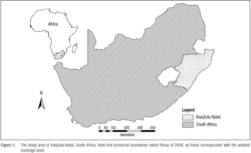
The study area covered the entire province of KwaZulu-Natal (KZN), which is located in the eastern central part of South Africa (Figure 1). The western boundary of the province is marked by the Drakensberg escarpment, which reaches over 3000 m amsl in places. The escarpment in the west and the warm Mozambique current in the east account for much of the large annual variation in temperature and rainfall experienced in the province.^22,23 Partly as a result of the varied geology, topography and climate (high mean annual precipitation and relatively low potential evapotranspiration) of the province²⁴, wetlands are well represented in this province, covering an area of at least 4200 km² (approximately 5% of KZN)²⁵. The hydrological regimes of wetlands in KZN are generally not only supplied by precipitation, but are also driven by a mixture of precipitation, groundwater (including infiltration, percolation and interflow) and streamflow. For example, the wetlands on the coastal plains owe their existence to the high rainfall averages and subtropical conditions as well as a series of marine regressions and transgressions that took place from 120 000 to 20 000 years BP²⁶ Conversely, high rainfall, gradual sediment trapping slopes and Karoo dolerite key points make areas climatically and geologically conducive to wetland formation inland. In KZN's escarpment areas, there is a high run-off of water which is collected in the topography of the landscape, and in cases in which the mean annual precipitation exceeds the potential evapotranspiration, the saturated soils remain wet - forming wetland rich areas. A second reason KZN was selected as a study area was that the province's array of diverse natural resources makes KZN suitable for varied agricultural production (mainly sugarcane, forestry and maize), mining activities and a variety of different domestic and industrial uses.²⁷ These activities are increasingly exerting pressure on the province's natural resources, including wetlands.

Model data

The initial step was to construct a data set of wetland presence/absence and associated environmental (landscape and climatic) variables^1,12 (Table 1). The existing wetland layer for KZN compiled by Scott-Shaw and Escott³³ represents the best available and most comprehensive wetland data set for the province, and was used as the basis for establishing wetland presence/absence. The provincial wetland layer is a compilation product that has been ongoing over the past decade, drawing from multiple sources, including the 1:250 000 geological map, the priority wetlands coverage identified by Begg³⁴, manual mapping using a wide variety of aerial and satellite imagery, and information collated from private sector sources. The wetland layer was split randomly using Hawth's tools³⁵ into training and test data sets to avoid over-fitting of the model³⁶. This wetland layer was used as the template for extracting environmental parameter statistics correlating with known wetland areas (training wetland data set), and to assess and validate the final probability layer output (test wetland data set). A key assumption was that the KZN wetland layer was accurate in terms of wetland extent area and location. To provide some level of confidence in the KZN wetland layer, an accuracy assessment of the layer was first completed before modelling began. Using 239 wetland sites from referenced aerial photographs,³⁷ the 2011 KZN wetland layer was visually assessed to determine if the coverage had captured their location and the extent of the wetland sites. The wetland layer correctly identified 82% (196 out of 239) of the photo reference wetland sites, providing a degree of confidence in the input wetland layer used in building and assessing the model. The 239 sites were identified from georeferenced large-scale aerial photographs, clearly identifying different wetland systems spread broadly across the entire province. These sites formed a part of a broader land-cover mapping field verification exercise, and therefore had no bias to the existing KZN wetland layer and were suitable for assessing and validating the wetland layer.

 

 

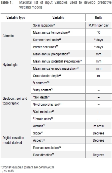
As the environmental variables associated with the wetlands layer differed in data format, spatial resolution, projection and extent because they were sourced from different organisations and institutions, standardisation of all input variables was required. Input variables that were model-derived had their own limitations and errors, and standardisation of these layers may have compounded these limitations; however, this possibility was unavoidable in this study. The initial step was to standardise the input variable layers in terms of projection, extent and format. The standardisation included the transformation of all layers to a common projection system (Transverse Mercator, WGS 84 datum), and resampling to a resolution of 20 m and an extent according to the digital elevation model (DEM)³² used in the model. Most layers were resampled from a coarser (± 30 m to 1600 m) to a finer (20 m) resolution using the nearest-neighbour resampling technique. This technique was chosen because it does not alter the cell values in the categorical variables during the resampling process.

Model development

The modelling process of the study was broken into a number of steps to derive the final raster layer representing the probability of wetland occurrence in KZN. The process made use of the geographical information system software package ArcGIS 9.3³⁸, statistical package R³⁹, the multivariate statistical package MVSP⁴⁰, NETICA⁴¹, and Medcalc⁴², with additional data manipulations performed in a spreadsheet. The basis for the modelling was a spreadsheet we generated of wetland presence and absence versus associated environmental variable values. This spreadsheet consisted of approximately 45 000 statistical extraction points (Hawth's tools was used to generate extraction points for non-wetland areas) to build the database, of which 25 000 were records for wetland presence and 20 000 for wetland absence.

Next, we investigated whether there were high levels of inter-correlation between the input predictor variables. From this analysis, we wanted to derive an optimal predictor data set by eliminating redundant variables for the original list of 19 possible variables. Principal component analysis (PCA)⁴⁰ was used to select an optimal set of input variables representing greater predictive power with regard to where wetlands are likely to occur. This approach of eliminating variables using PCA could only be processed using ordinal data, therefore excluding the nominal variables in this step, namely hydromorphic soils, geology and soil association. The process of elimination of redundancy involved the stepwise analysis of the biplots and variable loadings of each input variable. Correlation of two variables resulted in the elimination of the variable with the smallest variable loading. Preference was given to variables with higher spatial resolution. The co-linearity of the data set was tested following each rerun of the PCA, until the co-linearity of the data set was below the critical threshold value of ten.⁴³

Calculating probabilities for the BN required the data to be reduced to a finite set of mutually exclusive states (e.g. high, medium and low; yes or no).⁴⁴ Following this assumption, the refined pool of input variables was translated from continuous values to qualitative states of high, medium and low. Two approaches were used in discretising the data. Firstly, continuous data were reclassified into states using the Jenks natural break algorithm,⁴⁵ in which class breaks are identified that best group similar values and that maximise the differences between classes. Secondly, data in qualitative states were reclassified into states that best represented the respective variable characteristics; for example, the qualitative variable 'terrain units' discretised the states 'foot slope' and 'valley bottom' as low, 'mid-slope convex' and 'mid-slope concave' as medium and 'crest' as high. This reclassification was done for both the database and the corresponding spatial layers. Nominal variables that could not be quantified into qualitative states as required for the BN were eliminated from the model. Following the PCA elimination process and defining variable states, 'Hydromorphic Soils' was the only nominal variable added post PCA, for both models, because it could be discretised into 'yes' or 'no' states, signifying areas presumably well saturated under normal conditions, and thereby providing an additional predictor of wetland areas. Nominal variables made up of a number of nominal classes, such as soil association and geology, could not be discretised into states (high, medium or low). The discretising of variables into states with many nominal classes is a limitation of this method, and is a challenge of BNs in general.⁴⁶

We used NETICA⁴¹, which is the most popular BN software used in environmental modelling³⁶, to construct our BN model. The BN was structured using network nodes, each with a finite set of mutually exclusive states. Cain⁴⁴ explains that the links between these nodes represent their causal relationship, and each node has a set of probabilities specifying the likelihood that a node will be in a particular state given the states of those nodes that affect it directly.

Following the transformation of the input variables into states, the records in the database became cases in the case learning file for the BN, which produced conditional probabilities in a final conditional probability table (CPT), which in turn formed the basis in creating a wetland probability layer. BNs are informed through a set of cases (case learning file); in this instance, the training database represented the set of cases, and the number of cases represented the sample size.³⁶ Because BNs are not spatially explicit⁴⁷, a wetland probability layer had to be generated using the probabilities in the BN's CPT. The probability layer was derived by logarithmically coding the cases in both the CPT and the spatial input raster layers, so that values from the Bayesian CPT matched the equivalent logarithmic coded variable raster layers. The aggregation of the coded spatial layers created a single raster layer with unique logarithmic values as raster values. The aggregation of cases in the CPT created matching unique logarithmic values corresponding to probabilities. The unique logarithmic values with probabilities in the CPT formed the reclassification file, which was used to reclassify all the raster values in the raster layer to probabilities found in the CPT. This step created the probability layer, spatially indicating the probability of wetland occurrence in KZN. Probability values were then extracted using the test wetland and non-wetland point data set, which provided the necessary data for the receiver operating characteristic (ROC) analysis.

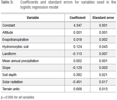
For a comparative approach, we used the same refined training wetland data set to fit a logit binomial model in the form of Equation 1 using a stepwise regression process.⁴⁸ The constant and variable coefficients calculated here were used to determine the probability of wetland occurrence at each wetland and non-wetland point in the binary test wetland data set. Model fitting was undertaken with the statistical package R³⁹ using the binary condition values (0, 1) as the response variable (generalised linear model, binomial distribution, logit link function³⁹) to estimate the probability of wetland occurrence. The LR model was made spatially explicit by multiplying the variable raster layers by their determined coefficients, and then adding all raster layers together into a single layer with the model constant added to the final layer.

where α is a constant and β is a coefficient for variable x, and where x could be, for example, the Landform type.

Model validation and assessment

The test wetland data set was used to compare the modelled probabilities derived from the LR model and the probabilities derived through a BN. ROC curves and the area under the curve (AUC) were used to compare the two models, and were calculated using suitable software.⁴² ROC analysis is a useful technique in visualising the performance of a binary classifier system as its discrimination threshold is varied. This variability provides a richer measure of classification performance than scalar measures such as accuracy, error rate and error cost.⁴⁹ In this instance, probabilities from the BN and LR model were assessed in approximately 8600 test wetland sites (derived from the test wetland data set), and in 8600 non-wetland sites (derived randomly using Hawth's tools). The 17 200 wetland and non-wetland sites formed the binary data necessary for the ROC analysis. The predicted probabilities from both models were plotted against each other to assess their degree of correlation. Key to this analysis was determining the sensitivity and specificity of the final probability layers at a criterion threshold as well as the AUC. The sensitivity defined how many positive results occurred among the 8600 test wetland sites (Equation 2) and the specificity defined how many correct negative results occurred among the 8600 non-wetland test sites (Equation 3).

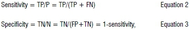
where P is positive and N is negative, TP is true positive and FP is false positive, and TN is true negative and FN is false negative.

To add to the comparison of the two models, we plotted a correlation between probabilities as outputs from each approach. This was further complemented and quantified using Cohen's kappa statistic to provide a statistical measure of agreement between the BN probability layer and the LR probability layer.⁵⁰ Using a determined threshold, the BN and LR probability outputs were transformed into two binary (wetland versus non-wetland) data sets for an agreement comparison.

To assess model usefulness for predicting wetland occurrence and extent, we generated 1000 random points across 20 classes of probability (i.e. 5-10%, 10-15%, 15-20%, etc.) and used Hawth's tools³⁵ to analyse the trend in accuracy in predicting wetland occurrence and extent. Wetland occurrence accuracy was determined by assessing whether a point occurred in a wetland area and confirmed using satellite imagery (Spot5 2009; Google Earth^TM). Here, each point was recorded as either falling within a wetland clearly identifiable on the imagery, or not, drawing on previous experience gained in desktop wetland delineation. The wetland extent accuracy was determined using the test wetland data set to obtain a probability value versus wetland extent area curve i.e. wetland extent area covered at increasing probability value intervals (i.e. 0-100%, 5-100%, 10-100%, etc.).

 

Results

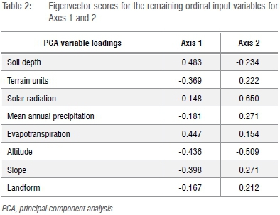
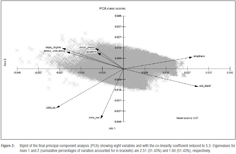
The maximal PCA accounted for 53.66% of the cumulative variance in axes 1, 2 and 3, with high levels of correlation (i.e. redundancy) between variables originally considered. The co-linearity condition number of the first PCA iteration was 37.9, exceeding the critical value of 10.0.³⁷ An example of this redundancy was the high correlation (r²<-0.9) between the clay and altitude variables. The clay variable was eliminated from the PCA as a result of this correlation, and because the altitude variable had a higher spatial resolution and accounted for more variation. Following the first iteration of the PCA, flow direction, flow accumulation, soil moisture and aspect (modified to ordinal variables) were eliminated because of their short vector length, which signifies only a small influence on the determination of wetland probability. In the second PCA iteration, the temperature variables (winter heat units, summer heat units, and mean annual temperature) were highly negatively correlated (r²<-0.9) with altitude, indicated by the ±180° angle separating the vectors. Because mean annual temperature accounted for more variation and had a higher spatial resolution, the additional temperature variables were eliminated. In the third PCA iteration, the biplot vectors of the groundwater and slope (DEM-derived³²) variables displayed virtually no angle between them (i.e. they were correlated), resulting in the elimination of groundwater because it was the variable with the shortest vector and smaller variable PCA loading. In the final PCA iteration, evaporation was highly correlated (r²=0.895) with the evapotranspiration variable. Evaporation was eliminated because it had the lower variable PCA loading of the two. Following the elimination of the evaporation variable, the data set's co-linearity condition number fell below the recommended critical threshold value.⁴³ After these iterations, the maximal data set was reduced to eight ordinal variables, with a resultant co-linearity condition number of 5.3. The final iteration of the PCA accounted for 69.15% of the cumulative variance in axes 1, 2 and 3 (Figure 2; Table 2), with the remaining input variables into the models being Mean Annual Precipitation, Slope (degrees), the 20-m DEM (hereafter referred to as 'Altitude'), Mean Annual Solar Radiation (hereafter referred to as Solar Radiation), Soil Depth, Evapotranspiration, Terrain Units and Landform. Following the PCA elimination process, Hydromorphic Soils was the only nominal variable added post-PCA. The final spreadsheet for both models was therefore based on a common predictor data set for nine variables (eight quantitative variables and one nominal variable).

 

 

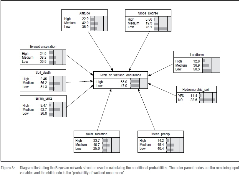
The BN model was informed by learning the cases in the database (case learning file) of the remaining input variables (Figure 3). The case learning file formed the central input for calculating the prior probabilities of all the parent node variables in the BN, as well as the final conditional probabilities. The output of the BN was a table with the conditional probabilities of wetland probability given the state of each input variable. The input variables reduced to qualitative states (high, medium, low) formed the parent nodes and the 'probability of wetland occurrence' formed the child node. The LR model to estimate probability of wetland occurrence (i.e. wetland = yes or no) was significant for all nine variables (p<0.05) (Table 3).

 

 

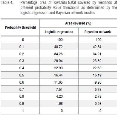
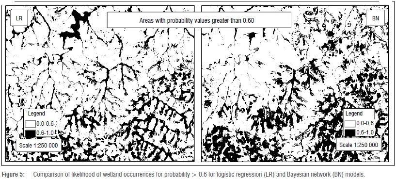
The final outputs of the BN and LR models were two raster layers with the pixel values representing probabilities of being a wetland at a spatial resolution of 20 m (Figure 4; Table 4). Probability values below 0.50 accounted for over 60% (~57 000 km²) of the total KZN area, while probability values of 0.80 and above accounted for only approximately 4-6% (3700-5500 km²) of the total KZN area (Table 4). The BN probability map appeared to be more conservative in estimating area than the LR map, for which, at a threshold of 0.6, the percentage area covered by the LR model was 0.88% more than the area covered by the BN model, even though probabilities from the BN and LR models were generally strongly correlated (r²=0.79). For Cohen's kappa statistic, both LR and BN layers were transformed into two binary data sets using a 0.6 probability cut-off. Based on Cohen's kappa result, observed and predicted wetland occurrences were more than 78% similar in all cases, with a 91% agreement between the LR- and the BN-derived probability layers (Figure 5).

 

 

Model validation and assessment

Results from the ROC curves indicated that the AUC for the predicted probabilities of the BN model and LR model were 0.853 (SE=0.00287; 95% confidence level = 0.847-0.858) and 0.840 (SE=0.00301; 95% confidence level = 0.835-0.846), respectively (Figure 6). An AUC of 1 indicates perfect prediction, whereas an AUC of 0.5 indicates completely random binary prediction. Although there was a marginal difference in the AUC results for the BN and LR models, the difference was not pronounced enough to conclusively state that one model has outperformed the other in predicting wetland occurrence. ROC analyses were performed using the test wetland data set to compare the predicted probabilities derived from a simple binary LR to the derived and predicted probabilities from the BN. The ROC analyses performed on the BN probability layer and the LR probability layer indicated that both models predicted the occurrence of wetlands relatively similarly⁵¹ (Figure 6). The ROC analysis determined that the criterion model probability threshold for both models (at which probability both the sensitivity (71.6) and specificity (81.2) are the highest as a pair) was greater than 0.60; i.e. if the probability values in both layers were split into binary classes of wetland and non-wetland areas, then 0.60 would be the ideal split to maintain good predictability of wetland and non-wetland occurrence.

 

 

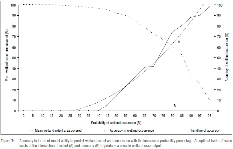
The trend analysis results indicated that there was a decreasing trend in accuracy of mean wetland extent area covered with an increase in probability of wetland occurrence (Figure 7). However, with the increase in probability, there was an increasing trend in accuracy of correctly predicting the presence of a wetland. The probable explanation for this trend is that the average wetland extent is made up of a mosaic of probability values, with the core being predicted by high probability values and the outer extents by lower probability values. Therefore lower probability ranges will occupy larger area extents but with a lower accuracy in identifying a single wetland area, whereas higher probability values will more likely identify wetland location but at the cost of accurately identifying the wetland's extent (Table 4).

 

Discussion

Current wetland mapping approaches are typically based either on aerial photography and/or satellite imagery interpretation or classification of satellite imagery, the latter involving complex methodologies utilising spectral ratios, indexes and values which are classified to identify wetland areas. It is common for wetland maps to under-represent certain areas for various reasons (errors, lack of resources, misclassification), and therefore these layers could help minimise these areas of under-representation. Consequently, resultant maps may suffer from pitfalls that include not linking wetland polygons that are fragments of larger wetland systems, and wetland omissions because of seasonal effects on satellite images. To compensate for these pitfalls, many methodologies draw support from ancillary data to improve the accuracy of wetlands mapped and classified.^14,18 Topological entities are commonly used as ancillary data and have been valuable in the success of many other wetland mapping approaches.^{5,14,18,52-55}

In this study, we assessed two methods that use topological and climatic variables as the basis for predicting the probability of wetland occurrence over a large spatial domain. The final wetland probability layers had good agreement with the current regional wetland layer and literature highlighting regional priority wetland areas.^26,34 Output layers indicated new areas of wetlands and how wetland fragments are likely to be part of larger but fragmented wetland systems. We acknowledge that using the PCA approach resulted in variables selected for the correlative rather than causative link to wetland presence. This was a necessary tradeoff that ignores the complexities and subtleties of topographic influence on wetland presence, but allows for greater objectivity and repeatability in model development; both methods do not require an understanding of the complex interactions and relationships of the environmental components that drive wetland formation and function. It is also to be expected that the models will predict different hydrogeomorphic wetland types with different levels of accuracy because of the different ways in which such environmental drivers interact, and at different scales, within the landscape. Moreover, the variables relevant to this model may not be entirely transferrable across different regions of South Africa because of possible differences in wetland ontology (geology, climate) between regions. A clear identified research need is therefore to establish suitable predictor variable sets across different climatic regions of South Africa, as the basis for developing regional probabilistic models.

There are advantages and limitations inherent in each approach. Uusitalo⁴⁶ reports that a BN can only deal with continuous data in a limited manner, and that there is no satisfactory automatic discretisation technique or method for data translation to qualitative states in BNs. The Jenks natural break interval method⁴⁵ was used to discretise the data into qualitative states in this study, but it is important that future researchers adopting this approach should pay careful attention when defining value ranges of continuous data to ensure that the intervals signify important breaks within data, so that the generalisation caused by discretisation is minimised. Conversely, the LR approach did not require the data to be discretised, and this method provided simpler and more integrated handling of continuous data than the BN approach. Given such tradeoffs, perhaps the most promising approach would be to use 'ensemble' or consensus modelling, in which the outputs of both models are combined such that the probabilities of occurrence of both algorithms are used to provide a combined output with a lower mean error.⁵⁶

The probability layers from either method have the potential to not only identify new wetland areas, but to guide the classification of satellite imagery by showing highly probable wetland areas, thereby avoiding the misclassification of pixels or the high errors associated with spectral confusion. However, we note that there will inevitably be trade-offs between the accuracy in the model's prediction of wetland extent and wetland occurrence. While the cut-off point for creating a useable wetland map is dependent on the user, we recommend 0.6 as a threshold for mapping probability only, but 0.8 when mapping extent and probability. For example, if the user is interested in using the model to identify new wetland areas, and is not concerned with the model's ability to predict wetland extent, the user would opt for a higher cut-off probability value, which produces a wetland map with a higher accuracy in predicting the wetland occurrence and a low accuracy in modelling the correct wetland extent. Using such ancillary data to support wetland mapping efforts has the potential not only to improve general land-cover assessments but also to better establish important spatial priorities for wetland conservation and management through improved conservation target estimation when measuring the current status of wetlands in an area in terms of wetland loss and current state of integrity. The final output has further applicability in already modified areas because the final model output predicts the likelihood of wetland occurrence regardless of any land-cover transformation. Predicted occurrence of wetlands without the effects of land transformation has implications both in establishing the historical extent of wetlands in regions of extensive land-cover transformation, as well as in establishing to what extent seemingly unrelated wetland polygons are in fact components of single larger systems now fragmented. We conclude that the methods assessed in this study have the potential to generate useful ancillary data to improve wetland mapping accuracy by identifying new wetland areas and providing insights on linkages between wetland fragments, but we recommend further ground truthing to assess such layers. From a pragmatic and computational perspective, our preference would be to use the LR approach as the basis for developing regional wetland probability maps for additional regions in South Africa.

 

Acknowledgements

We thank the Mondi Wetland Programme for funding this research, and Dr Boyd Escott (Ezemvelo KZN Wildlife) and the Agricultural Research Council: Institute for Soil, Climate and Water for providing spatial data relating to wetlands in KwaZulu-Natal. We sincerely thank the two reviewers for their comments and inputs into the manuscript.

 

Authors' contributions

N.R.M. was the project supervisor and conceptualised the study. J.H. performed the majority of the data analyses and all of the GIS analyses as part of his MSc study at UKZN. N.R.M. and J.H. wrote the manuscript.

 

References

1. Mitsch WJ, Gosselink JG. Wetlands. 3rd ed. New York: John Wiley & Sons Inc.; 2000.         [ Links ]

2. Woodhouse S, Lovett A, Dolman P Fuller R. Using GIS to select priority areas for conservation. Comput Environ Urban Sys. 2000;24:79-93. http://dx.doi.org/10.1016/S0198-9715(99)00046-0        [ Links ]

3. May D, Wang J, Kovacs J, Mutter M. Mapping wetland extent using IKONOS satellite imagery of the O'donell point region, Georgian Bay, Ontario. London, Ontario: University of Western Ontario; 2002.         [ Links ]

4. Chhokar KB, Pandya M, Raghunathan M. Understanding environment. New Delhi: Sage Publications India Pvt; 2004.         [ Links ]

5. Islam MA, Thenkabail PS, Kulawardana RW, Alankara R, Gunasinghe S, Edussriya C, et al. Semi-automated methods for mapping wetlands using Landsat ETM+ and SRTM data. Int J Remote Sens. 2008;29:7077-7106. http://dx.doi.org/10.1080/01431160802235878        [ Links ]

6. Millennium Ecosystem Assessment (MEA). Ecosystem and human well-being: Wetlands and water synthesis. Washington DC: World Resources Institute; 2005.         [ Links ]

7. Ramsar Convention Secretariat. Ramsar handbooks for the wise use of wetlands. 4th ed. Gland: Ramsar Convention Secretariat; 2010.         [ Links ]

8. Olhan E, Gun S, Ataseven Y Arisoy H. Effects of agricultural activities in Seyfe wetland. Sci Res Essays. 2010;5:9-14.         [ Links ]

9. Ozesmi SL, Bauer ME. Satellite remote sensing of wetlands. Wetl Ecol Manag. 2002;10:381-402. http://dx.doi.org/10.1023/A:1020908432489        [ Links ]

10. Adam E, Mutanga O, Rugege D. Multispectral and hyperspectral remote sensing for identification and mapping of wetland vegetation: A review. Wetl Ecol Manag. 2010;18:281-296. http://dx.doi.org/10.1007/s11273-009-9169-z        [ Links ]

11. Wilen BO, Carter V Jones JR. Wetland management and research: Wetland mapping and inventory. National Water Summary on Wetland Resources, US Geological Survey Water Supply Paper 2425 [homepage on the Internet].         [ Links ] c2002 [cited 2015 June 17]. Available from: https://water.usgs.gov/nwsum/WSP2425/mapping.html

12. Batzer, DP, Sharitz, RR, editors. Ecology of freshwater and estuarine wetlands. Berkeley, CA: University of California Press; 2006.         [ Links ]

13. Yu H, Zhang S. Application of high resolution satellite imagery for wetlands cover classification using object-oriented method. Int Arch Photogramm Remote Sens. 2008;XXXVII(B7):521-526.         [ Links ]

14. Kulawardhana RW, Thenkabail PS, Vithanage J, Biradar C, Islam MA, Gunasinghe S, et al. Evaluation of the wetland mapping methods using Landsat ETM+ and SRTM data. J Spat Hydrol. 2007;7:62-96.         [ Links ]

15. Rebelo LM, Finlayson CM, Nagabhatla N. Remote sensing and GIS for wetland inventory, mapping and change analysis. J Environ Manage. 2009;90:2144-2153. http://dx.doi.org/10.1016/j.jenvman.2007.06.027        [ Links ]

16. Knight AW, Tindall DR, Wilson BA. A multitemporal multiple density slice method for wetland mapping across the state of Queensland, Australia. Int J Remote Sens. 2009;30:3365-3392. http://dx.doi.org/10.1080/01431160802562180        [ Links ]

17. Landmann T, Schramm M, Colditz RR, Dietz A, Dech S. Wide area wetland mapping in semi-arid Africa using 250-meter MODIS metrics and topographic variables. Remote Sens. 2010;2:1751-1766. http://dx.doi.org/10.3390/rs2071751        [ Links ]

18. Li J, Chen W. A rule-based method for mapping Canada's wetlands using optical, radar and DEM data. Int J Remote Sens. 2005;26:5051-5069. http://dx.doi.org/10.1080/01431160500166516        [ Links ]

19. Lunetta RS, Balogh ME, Merchant JW. Application of multi-temporal Landsat 5 TM imagery for wetland identification. Photogramm Eng Remote Sens. 1999;65:1303-1310.         [ Links ]

20. Ryo M, Peng G, Bing X. Spectral mixture analysis for bi-sensor wetland mapping using Landsat TM and Terra MODIS data. Int J Remote Sens. 2012;30:3373-3401.         [ Links ]

21. Ricchetti E. Multispectral satellite image and ancillary data integration for geological classification. Photogramm Eng Remote Sens. 2000;66:429-435.         [ Links ]

22. Allen, KM, Green SW, Zubrow EB. Interpreting space: GIS and archaeology. London: Taylor and Francis; 1990.         [ Links ]

23. Eeley HAC, Lawes MJ, Piper SE. The influence of climate change on the distribution of indigenous forest in KwaZulu-Natal, South Africa. J Biogeogr. 1999;26:595-617. http://dx.doi.org/10.1046/j.1365-2699.1999.00307.x        [ Links ]

24. King L. A geomorphology of central and southern Africa. Biogeography and ecology of southern Africa. Monogr Biol. 1978;31:1-17. http://dx.doi.org/10.1007/978-94-009-9951-0_1        [ Links ]

25. Rivers-Moore NA, Cowden C. Regional prediction of wetland degradation in South Africa. Wetl Ecol Manag. 2012;20:1-14. http://dx.doi.org/10.1007/s11273-012-9271-5        [ Links ]

26. Patrick MJ, Ellery WN. Plant community and landscape patterns of a floodplain wetland in Maputaland, Northern KwaZulu-Natal, South Africa. Afr J Ecol. 2006;45:175-183. http://dx.doi.org/10.1111/j.1365-2028.2006.00694.x        [ Links ]

27. KwaZulu-Natal Provincial Planning Commission (KZNPPC). Provincial growth and development strategy. Pietermaritzburg: KZNPPC; 2011.         [ Links ]

28. Schulze RE. South African atlas of agrohydrology and climatology. Report TT82/96. Pretoria: Water Research Commission; 1997.         [ Links ]

29. Colvin C, Le Maitre D, Saayman I, Hughes S. Introduction to aquifer dependent ecosystems in South Africa. Pretoria: Natural Resources and the Environment, CSIR; 2007.         [ Links ]

30. Escott B. Landform map for KZN based on the 90m SRTM DEM (v4 edited). Pietermaritzburg: Ezemvelo KZN Wildlife; 2011.         [ Links ]

31. Van den Berg HM, Weepener HL, Metz M. Spatial modeling for semi-detailed soil mapping in KwaZulu-Natal. Report No: GW/A/2009/48. Pretoria: Agricultural Research Council - Institute for Soil, Climate and Water; 2009.         [ Links ]

32. GISCOE 20m GISCOE DTM Data. Pretoria: GISCOE Pty Ltd; 2001.         [ Links ]

33. Scott-Shaw CR, Escott BJ. KwaZulu-Natal provincial pre-transformation vegetation type map 2011. Pietermaritzburg: Biodiversity Conservation Planning Division, Ezemvelo KZN Wildlife; 2011 [unpublished].         [ Links ]

34. Begg GW. The wetlands of Natal part 3: The location, status and function of the priority wetlands of Natal, report 73. Pietermaritzburg: Natal Town and Regional Planning Commission; 1989.         [ Links ]

35. Beyer HL. Hawth's analysis tools for ArcGIS [homepage on the Internet]. c2004 [cited 2011 May 22].         [ Links ] Available from: http://www.spatialecology.com/htools/

36. Aguilera PA, Fernandez A, Fernandez R, Rumi R, Salmeron A. Bayesian networks in environmental modelling. Environ Model Softw. 2011;26:1376-1388. http://dx.doi.org/10.1016/j.envsoft.2011.06.004        [ Links ]

37. Jewitt D. Landcover accuracy assessment photography 2011. Pietermaritzburg: Biodiversity Research and Assessment Division, Ezemvelo KZN Wildlife; 2011 [unpublished].         [ Links ]

38. Environmental Systems Research Institute (ESRI). ArcGIS desktop release 9.3. Redlands, CA: ESRI; 2007.         [ Links ]

39. R Development Core Team. R: A language and environment for statistical computing. Vienna: R Foundation for Statistical Computing; 2009. Available from: http://www.R-project.org        [ Links ]

40. Kovach WL. MVSP: A multivariate statistical package for Windows version 3.2. Pentraeth, Wales: Kovach Computing Services; 1999.         [ Links ]

41. Netica version 4.10. Vancouver: Norsys; 2010. Available from: www.norsys.com        [ Links ]

42. MedCalc for Windows version 12.5. Ostend, Belgium: MedCalc Software; 2013. Available from: www.medcalc.org        [ Links ]

43. Fry JC. Biological data analysis. New York: Oxford University Press; 1993.         [ Links ]

44. Cain J. Planning improvements in natural resources management: Guidelines for using Bayesian networks to support the planning and management of development programmes in the water sector and beyond. Wallingford, UK: Centre for Ecology & Hydrology; 2001.         [ Links ]

45. Jenks GF, Caspall FC. Error on chloroplethic maps: Definition, measurement, reduction. Ann Amer Geogr. 1971;61:217-244. http://dx.doi.org/10.1111/j.1467-8306.1971.tb00779.x        [ Links ]

46. Uusitalo L. Advantages and challenges of Bayesian networks in environmental modelling. Ecol Model. 2007;203:312-318. http://dx.doi.org/10.1016/j.ecolmodel.2006.11.033        [ Links ]

47. Grêt-Regmey A, Straub D. Spatially explicit avalanche risk assessment linking Bayesian networks to GIS. Nat Hazards Earth Syst Sci. 2006;6:911-926. http://dx.doi.org/10.5194/nhess-6-911-2006        [ Links ]

48. Crawley MJ. The R book. Chichester: John Wiley & Sons Ltd; 2007.         [ Links ]

49. Fawcett T. An introduction to ROC analysis. Pattern Recogn Lett. 2006;27:861-874. http://dx.doi.org/10.1016/j.patrec.2005.10.010        [ Links ]

50. Carletta J. Assessing agreement on classification tasks: The kappa statistic. Comput Ling. 1996;22:249-254.         [ Links ]

51. Zhou XH, Obuchowski NA, McClish DK. Statistical methods in diagnostic medicine. New York: Wiley; 2002. http://dx.doi.org/10.1002/9780470317082        [ Links ]

52. Ibrahim K. Assessment of wetlands in Kuala Terengganu District using Landsat TM. J Geogr Geol. 2009;1:33-40. http://dx.doi.org/10.5539/jgg.v1n2p33        [ Links ]

53. Bwangoy JB, Hansen MC, Roy DP Grandi G, Justice CO. Wetland mapping in the Congo Basin using optical and radar remotely sensed data and topographical indices. Remote Sens Environ. 2010;114:73-86. http://dx.doi.org/10.1016/j.rse.2009.08.004        [ Links ]

54. Pantaleoni E, Wynne RH, Galbraith JM, Campbell JB. A logit model for predicting wetland location using RASTER and GIS. Int J Remote Sens. 2009;30:2215-2236. http://dx.doi.org/10.1080/01431160802549310        [ Links ]

55. Wright C, Gallant A. Improved wetland remote sensing in Yellowstone National Park using classification trees to combine TM imagery and ancillary environmental data. Remote Sens Environ. 2007;107:582-605. http://dx.doi.org/10.1016/j.rse.2006.10.019        [ Links ]

56. Araújo MB, New M. Ensemble forecasting of species distributions. Trends Ecol Evol. 2007;22:42-47. http://dx.doi.org/10.1016/j.tree.2006.09.010        [ Links ]

 

 

Correspondence:
Nick Rivers-Moore
Centre for Water Resources
Research, University of KwaZulu-Natal
Private Bag X01,Scottsville 3209
South Africa
Email: blackfly1@vodamail.co.za

Received: 30 May 2014
Revised: 26 Aug. 2014
Accepted: 16 Sep. 2014