RESEARCH ARTICLE

 

Impact of lower stratospheric ozone on seasonal prediction systems

 

 

Kelebogile Mathole^I; Thando Ndarana^I; Asmerom Beraki^I; Willem A. Landman^{II, III}

^ISouth African Weather Service -Research, Pretoria, South Africa
^IICouncil for Scientific and Industrial Research - Natural Resources and the Environment, Pretoria, South Africa
^IIIDepartment of Geography, Geoinformatics and Meteorology, University of Pretoria, Pretoria, South Africa

Correspondence

 

 

---

ABSTRACT

We conducted a comparison of trends in lower stratospheric temperatures and summer zonal wind fields based on 27 years of reanalysis data and output from hindcast simulations using a coupled ocean-atmospheric general circulation model (OAGCM). Lower stratospheric ozone in the OAGCM was relaxed to the observed climatology and increasing greenhouse gas concentrations were neglected. In the reanalysis, lower stratospheric ozone fields were better represented than in the OAGCM. The spring lower stratospheric/ upper tropospheric cooling in the polar cap observed in the reanalysis, which is caused by a direct ozone depletion in the past two decades and is in agreement with previous studies, did not appear in the OAGCM. The corresponding summer tropospheric response also differed between data sets. In the reanalysis, a statistically significant poleward trend of the summer jet position was found, whereas no such trend was found in the OAGCM. Furthermore, the jet position in the reanalysis exhibited larger interannual variability than that in the OAGCM. We conclude that these differences are caused by the absence of long-term lower stratospheric ozone changes in the OAGCM. Improper representation or non-inclusion of such ozone variability in a prediction model could adversely affect the accuracy of the predictability of summer rainfall forecasts over South Africa.

Keywords: polar vortex; eddy-driven jet; stratosphere; ozone depletion; ENSO

---

 

 

Introduction

The El Nino Southern Oscillation (ENSO) phenomenon is the single biggest contributing factor to climate variability because of its large global impact.¹ Its effect on seasonal summer rainfall over South Africa is well documented.^2-4 Studies have shown that ENSO signals are usually associated with rainfall anomalies over the country, that is, above normal rainfall conditions are often associated with La Nina events and below normal rainfall with El Nino events. ENSO-forced predictability becomes even more enhanced during the austral summer as a result of tropical circulation that becomes dominant during this season and thus increases the predictability of rainfall at shorter lead time scales.⁵ Moreover, numerous modelling studies^5,6 have shown that variations of sea surface temperatures from the equatorial Pacific and Indian Oceans provide skillful predictions over southern Africa because of the linear relationship that they have with the region's summer seasonal rainfall.⁷ Therefore, ENSO serves as a source for seasonal predictability over southern Africa, particularly in the case of above normal summer rainfall during La Nina years.⁸

Although ENSO-based seasonal prediction systems have come a long way to produce skillful summer rainfall forecasts during La Nina and El Nino events, they are constrained during neutral conditions over the equatorial Pacific Ocean as their skill diminishes.⁹ Furthermore, ENSO explains only about 20-30% of the climate variability¹⁰ over southern Africa. Stratosphere/troposphere coupling and stratospheric dynamics could therefore be explored and added as sources of seasonal predictability for the region; this notion is explored in this paper.

The eddy-driven jet, which dominates the circulation over the southern hemisphere during the summer,¹¹ and the associated storm tracks affect summer rainfall over South Africa.¹² The mechanism which is responsible for this association is explained by low-level baroclinicity.¹³ An anomalously poleward position of the jet and storm tracks is associated with anomalously wet conditions over South Africa and an anomalously equatorward position is associated with anomalously dry conditions. During anomalously dry conditions, the cloud bands that bring much of the country's summer rainfall are displaced from their usual position and are located east of the country. Because the position of the jet is influenced by the strength of the polar vortex^14,15 through robust stratospheric and tropospheric coupling mechanisms, the variability of winter and spring stratospheric winds, as well as temperatures, could be a source of summer rainfall predictability.¹⁶ Moreover, Son et al.¹⁷ have shown that for stratospheric variability to be useful in predicting tropospheric processes, the former has to be represented correctly in a model.

At longer timescales, observational¹⁸ and modelling studies^17,19 have shown that the formation of the ozone hole has led to lower stratospheric and upper tropospheric cooling during the austral spring months. This formation has also been responsible for the persistent poleward movement of the eddy-driven jet during the summer and a persistent positive phase of the Southern Annular Mode.²⁰ As would be expected, these changes in the tropospheric circulations have been accompanied by long-term changes in subtropical rainfall patterns.^21,22 However, these changes have not been caused by ozone depletion alone. Increasing greenhouse gas (GHG) concentrations have a cooling effect on the lower stratosphere.²³ During the 1970s to 2000, these two radiative forcings complemented each other.²⁴

Because summer rainfall over South Africa is influenced by the interannual variability of the position of the jet,¹² it is reasonable to hypothesise that a model that incorrectly simulates the jet position variability and climatology will likely be unable to simulate rainfall variability correctly. The effect may subsequently compromise the reliability of rainfall predictions at the seasonal timescale, but improved representation of stratospheric processes - such as ozone depletion - in climate models used to predict climate variability might lead to improved seasonal forecasts.

The representation of stratospheric processes in climate models has various facets and is important for realistic simulations. A recent study²⁵ showed that if ozone variations in a model are zonally symmetrical as opposed to three dimensional, lower stratospheric and upper tropospheric temperature trends as well as changes in the zonal winds are underestimated. The proper representation of stratospheric ozone is achieved through the use of interactive stratospheric chemistry schemes such as McLandress et al.'s¹⁹. It is also possible that the atmospheric level at which the model top is located plays an important role in the accuracy of climate models in simulating stratospheric dynamics. The highest level in most models is 10 hPa, which is far too low to accurately capture the stratospheric polar vortex.

Information on stratospheric processes that occur at levels higher than 10 hPa is conveyed into the model vertical domain by specifying model top boundary conditions.²⁶ However, these boundary conditions may not be equivalent to actually including the stratospheric processes, which can be achieved by raising the model top to 0.01 hPa. An idealised modelling study²⁷ showed that stratospheric/tropospheric coupling is captured clearly in a model with the top as high as 0.1 hPa. High top models are also considered in CMIP5.²⁸ Increasing stratospheric resolution, in addition to the above, has the ability to improve seasonal climate predictions significantly.²⁹ Studies such as Roff et al.'s³⁰ also indicate the importance of stratospheric resolution on extended forecasting skill. All these issues are applicable at timescales longer than that of seasonal prediction but are relevant to this timescale and therefore raise many questions with regard to the role of stratospheric processes and seasonal predictability. As such, in this paper we consider the behaviour of lower stratospheric and upper tropospheric temperatures, as well as that of the eddy-driven jet of a coupled ocean-atmosphere general circulation model (OAGCM) in which the ozone representation is not realistic and has no GHG forcing. We then compare this behaviour to reanalysis data. This effort is to highlight the implications of forcing a seasonal prediction model with climatological stratospheric ozone fields that are zonally averaged.

 

Data and methods

We obtained hindcasts from the South African version of the coupled European Centre Hamburg Model (version 4.5) - Modular Ocean Model, version 3-South Africa, Ocean Atmosphere General Circulation Model (called the ECHAM 4.5-MOM3-SA OAGCM)³¹ integrations for the first lead time (i.e. forecasts are made in early November for December-January-February).This model currently is used for operational forecast production at the South African Weather Service. Daily averages of zonal wind velocity and temperature fields over a period of 27 years (1983-2009) were constructed for the analyses. The coupled model output is available at a T42 (triangular truncation at wave number 42) horizontal resolution corresponding to a grid with 64 latitudes and 128 longitudes and with 19 vertical levels. The ozone field in the coupled model is relaxed toward the observed climatology and the anthropogenic forcing is neglected. The data set used here as a proxy for observation is from the National Centre for Environmental Prediction (NCEP) of the Department of Energy Reanalysis II³² which is an updated version of the original NCEP data set.³³ Fixed fields such as lower stratospheric ozone and carbon dioxide (CO₂) concentrations have been improved. Seasonal climatology ozone is used in the radiation calculations to better represent processes associated with it. Therefore ozone depletion and increasing CO₂ are both presented more realistically than previously. NCEP reanalysis has a typical horizontal resolution of 73 latitude grids and 144 longitude grids (2.5° x 2.5°) with 17 vertical levels.

Using the two data sets (coupled model hindcasts and NCEP reanalysis), we investigated the hypothesis that lower stratospheric cooling is influenced by short-term variations and depletion in ozone. Linear trends were calculated by fitting least squares regression curves onto both data sets and then comparing them. The jet location was obtained by first calculating the zonal average of the zonal wind fields and then fitting cubic splines at all pressure levels followed by identifying the maximum value of the zonal wind over the whole of the troposphere. This approach bypasses problems associated with variations in the level at which the maximum zonal wind value occurs.

 

Climatology of the zonal wind

Figure 1a and 1b show the climatological general structure of the zonal wind flow during austral summer (DJF) as a function of latitude and pressure for both observations and coupled model hindcasts, respectively. This structure is characterised by positive westerlies covering the tropospheric region (within the 850 hPa and 10 hPa levels), with a strong wind maximum that is associated with the eddy-driven jet. The jet core in the observations and in the model occur at different levels. It is lower, located at 350 hPa, in the former but is higher than 350 hPa in the OAGCM. These zonal wind structures are caused by the strong meridional temperature gradient found in the middle latitudes, as required by the thermal wind balance.³⁴ The meridional temperature gradient is in turn caused by differential heating between the tropical and polar regions. Eddy momentum fluxes that converge in the middle latitudes³⁵ are responsible for maintaining the jet after having been transported poleward by anti-cyclonically breaking upper tropospheric troughs^34,36,37. Also at play are energy conversions - barotropic processes that are associated with breaking waves convert eddy kinetic energy to mean kinetic energy.³⁴

There also are significant differences between the NCEP and OAGCM jet structures (Figure 1a and 1b). The former shows a weaker jet core which is centred more poleward (at about 48°S) than its OAGCM counterpart (at about 42°S). However, the jet in the model appears to be more elevated than in the reanalysis, which could also have implications for moisture transport. As was alluded to in the introduction and will be discussed further below, the climatological position of the jet should be an important consideration in seasonal prediction systems because it determines the short-term (interannual) variability of the jet's position relative to South Africa. The position of the summer jet in the different data sets also indicates that the storm tracks would be placed at different locations in the observations and in the model. The association between the eddy-driven jet and storm tracks occurs through baroclinic waves which influence the zonal mean flow and hence storm tracks activity.³⁸ Storm tracks are important because they transport heat, moisture and momentum.³⁹

Figure 1c and 1d give an indication of a relative climatological stratospheric wind circulation during austral winter (JJA) and spring (SON), respectively. These figures show zonal winds at 10 hPa, a level which is considered to be in the lower stratosphere as it is above the 500 K isentropic level for both data sets. Various studies^40,41 have used potential vorticity at this isentropic level to diagnose the dynamics of the polar vortex. A typical vortex comprises strong winter westerly winds replacing the summer and autumn easterlies.⁴² The vortex decays in late spring and the timing of its break up is highly variable.^40,42

The peaks of the winds at 10 hPa that occur in the mid-latitudes in Figure 1c and 1d are a good indication of the lower stratospheric polar night jet ⁴³ in the data sets considered here⁴⁴, hence the associated polar vortex. NCEP climatological winds at 10 hPa are stronger than in the OAGCM case during the winter and spring. As noted above, a persistent stronger (or weaker) polar vortex during the winter and, in particular, spring, leads to a poleward (or equatorward) eddy-driven jet during summer.^14,15 Therefore, because the NCEP vortex is stronger than its OAGCM counterpart, one would expect the summer eddy-driven jet of the former to be positioned more poleward than that of the OAGCM. This displacement is indeed found to be the case. This effect is a purely dynamical phenomenon as it has been demonstrated by idealised modelling studies.¹⁴ Idealised models comprise only dynamical cores and other physical processes⁴⁴ to separate atmospheric dynamical phenomena from other processes. The above discussion suggests that the climatology of stratospheric zonal winds is consistent with the tropospheric circulation in both data sets.

 

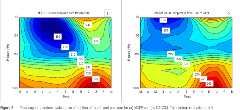
Evolution of polar cap temperatures

We now consider the climatological evolution of polar cap temperatures. They are defined as zonally averaged (longitude is considered negligible) temperature fields that are also averaged from 70° to 90°S. The selection of this latitude range confirms the south polar cap and defining the polar cap in this way is common practice.^25,45 Figure 2a and 2b show the polar cap temperature for the NCEP and OAGCM, as a function of month and pressure level. The evolution of lower tropospheric polar cap temperatures is similar in NCEP and OAGCM, but both the lower stratosphere and upper troposphere are quite different. The structure of the changes of NCEP temperatures are consistent with those of ozone concentrations as seen in Atmospheric Chemistry and Climate (AC&C) and Stratospheric Processes And their Role in Climate (SPARC) data (Figure 1).⁴⁵ Because lower stratospheric ozone has not depleted in the OAGCM, as opposed to in NCEP reanalysis which has a better representation of ozone, the lower stratosphere of the former is much warmer than that of the latter. By the thermal wind relation³⁴ one can see why the NCEP polar vortex is stronger than its OAGCM counterpart (Figure 1).

These results reveal that the NCEP climatological structure of the zonal wind distribution in the lower stratosphere during winter and the associated summer zonal wind distribution throughout the tropospheric mid-latitude regions are different from those of the OAGCM. The relative strengths of the polar night jet in the respective data sets are also consistent with the climatological temperatures in the lower stratosphere and upper troposphere, which in turn are consistent with ozone representation in the data sets.

 

Seasonal trends

In the discussion above we demonstrated that there are significant differences between the mean stratospheric and mean tropospheric winds and temperatures during the winter, summer and spring seasons in NCEP and OAGCM data. It was further suggested that this finding might be linked to the inadequate radiative forcing in the OAGCM, which may be caused by unrealistic ozone variations. In this section we consider the changes in the lower stratospheric temperatures during the spring season in the different data sets and their associated tropospheric response during the summer months, as established in previous modelling and observation studies. This work is aimed at demonstrating the likely importance of proper radiative forcing representation in seasonal prediction systems. The polar cap stratosphere is climatologically colder in the NCEP case than in the OAGCM, as noted above.³⁴

These climatological thermal structures could be associated with changes in the temperatures. As shown in Figure 3a, NCEP polar cap temperature exhibits cooling in the lower stratosphere and upper troposphere during October to March. This result is consistent with observational studies¹⁸ which used radiosonde data sets and model simulations^19,25 using chemistry climate models with state-of-the-art interactive stratospheric chemistry schemes. As shown in these studies and others, this cooling is a direct result of ozone depletion with increasing GHG concentrations augmenting it.¹⁷ There is no such cooling in the OAGCM polar cap (Figure 3b). The reason for this absence of cooling is that the ozone does not deplete in the model because, as noted previously, it is represented as monthly climatologies. Furthermore, the GHG concentrations do not increase in the OAGCM. Figure 3c shows the corresponding linear trends in NCEP zonal winds averaged between 50°S and 70°S as a function of month. The zonal wind response to the cooling begins during October in the lower stratosphere and upper troposphere. This response is shown by positive linear trends and it is most evident in the middle and lower troposphere during the summer months (Figure 3c) - a phenomenon that is well documented. As expected, a similar response does not occur in the OAGCM. Instead, there is a negative trend in the zonal wind between 50°S and 70°S in the OAGCM (Figure 3d). This result suggests (as will be further elaborated on below) that the tropospheric response in the model, although consistent with the associated polar cap temperatures, is not realistic.

 

Impact of ozone concentration

It has been demonstrated in Figure 3 that when ozone variations are represented in a realistic manner (meaning that ozone depletion actually occurs in the NCEP data sets), then the stratospheric cooling that results from ozone depletion has a tropospheric response that is particularly evident during austral summer. If this is not the case, as shown by the coupled model, ozone does not deplete and thus an opposite tropospheric response occurs. These features are shown as positive and negative linear trends represented by thin black and red contours, respectively (Figure 4a and 4b). This tropospheric response is actually an acceleration (or deceleration) of the eddy-driven jet on the poleward (or equatorward) side and is shown in Figure 4a. This response is consistent with what is seen in Figure 3c, which shows positive linear trends as a result of stratospheric cooling caused by ozone depletion (Figure 3a). A response in December-January-February mainly occurs as a result of stratospheric anomalies that have a time lag of a few months to descend to the surface.^18,46

The linear trends are a manifestation of the poleward movement of the eddy-driven jet as shown by the red linear trend line in Figure 4c, which moved from about 46°S to about 50°S during the analysed period. As noted before, the shift in the jet is a result of a cooler ozone-induced polar stratosphere (Figure 3a). A Monte Carlo or re-randomisation test^47,48 was performed on the reanalysis data linear trend of Figure 4c to test for its statistical significance by randomly creating a time series from the original interannual NCEP variations. After each re-randomisation, a least squares regression line was fitted to the randomised data from which the trend was calculated, and the process was repeated 10 000 times. The number of times the original trend was larger than the re-randomised trends was noted. Less than 1% of the re-randomised trends were larger than the original trend. This sloping linear fit is therefore statistically significant at the 99% level of confidence.

The magnitude of the poleward shift can also be measured using the climatological position as a reference (green straight line in Figure 4c). The initial sub-climatological jet position was equatorward of the climatological position and ended up on the poleward side of it at the end of the study period. The OAGCM jet tended to decelerate (accelerate) on the poleward (equatorward) side, although this tendency was weak (Figure 4b). The response of the jet in Figure 4b is also consistent with the tropospheric response seen in Figure 3d. These responses are a result of the warm stratosphere caused by the non-depletion of ozone. Moreover, this weak tropospheric response has resulted in the lack of trends shown by the black straight line coinciding with the climatological jet position in Figure 4c. It is clear that there are notable differences between NCEP and OAGCM lower stratospheric cooling during the spring and the associated summer tropospheric response to that cooling.

To conclude, we point to the possible importance of the proper lower stratospheric ozone variations to seasonal prediction by considering the interannual variability of the position of the jet. As noted in the introduction, variations of the jet position relative to South Africa are important to the country's summer rainfall. Most of the summer rainfall results from long cloud bands that stretch diagonally across the mainland and connect the tropical processes to the mid-latitudes through tropical temperate troughs.⁴⁹ When the eddy-driven jet is placed anomalously equatorward, these cloud bands become displaced and occur outside the eastern boundaries of South Africa, which leads to a dry summer season.¹²

 

Summary and conclusions

It has been demonstrated that in an OAGCM that has a climatological representation of lower stratospheric ozone, the depletion thereof (as opposed to in the reanalysis data) does not occur. The non-depletion of ozone leads to a lack of stratospheric temperature cooling, in contrast with the findings of previous studies^18,19,25 that have shown that ozone depletion leads to the cooling of the lower stratosphere. The reanalysis data show a significant austral summer tropospheric response that manifests as an acceleration of the eddy-driven jet on the poleward side and its deceleration on the equatorward side. These features are caused by a gradual and persistent poleward migration of the sub-climatological jet core. Because of the lack of ozone depletion in the OAGCM, the same is not observed. Instead, the sub-climatological jet remains largely stationary as indicated by the weak acceleration and deceleration of the climatological jet stream on the equatorward and poleward sides, respectively. However, the aim of this study was to demonstrate that the exclusion of long-term changes in stratospheric ozone (and GHGs) leads to an inaccurate position of the jet stream and the interannual vacillations of the zonal wind fields occur about an inaccurate latitude in the OAGCM - far more north than where it is supposed to be. However, the phases of the zonal wind anomalies observed in the NCEP reanalysis were correctly reproduced by the OAGCM, suggesting that the model simulated the ENSO signal correctly. The issue of stratospheric wind and temperature anomalies as a source at seasonal predictability under realistic ozone prescription and anthropogenic forcing is beyond the scope of this paper and is currently under investigation.

Whilst the trends in the jet position are associated with ozone depletion, and therefore apply to longer-term stratospheric/tropospheric dynamical coupling, they could also be important for seasonal prediction because South African summer rainfall is regulated by the position of the eddy-driven jet and associated storm tracks, relative to the land.¹² If the jet is placed more poleward than usual, then the country experiences a wet summer season. Otherwise the cloud bands which result in most of the summer rainfall are displaced eastward, leading to a dry summer. Therefore, the ozone depletion induced poleward trends of the jet position (as is observed to be the case in the reanalysis data sets) would affect interannual seasonal rainfall occurrence over South Africa and cause the low frequency vacillations of the jet to be progressively poleward. Other mechanisms such as stratospheric-tropospheric exchange could also influence the movement of this jet because its chemical effect in turn influences the lower stratosphere.⁵⁰ However, the exact mechanism by which the stratosphere influences the troposphere is unknown and still is under investigation.¹⁴ In fact, the study by Kang et al.²¹ found a direct link between changes in summer rainfall in the subtropical belt and the ozone hole, thus attesting to the importance of this forcing. As there is no such poleward trend in the OAGCM used in this study, its simulation of rainfall cannot be expected to be completely realistic. One way of improving this state of affairs is to improve representation of lower stratospheric ozone as well as GHG concentrations in models. The latter is important in this respect as it cools the lower stratosphere, albeit to a much lesser extent than the ozone hole formation. Advanced modelling centres such as the Canadian Climate Modeling Centre⁵¹ and the National Aeronautics and Space Administration⁵² employ interactive stratospheric chemistry. Such configurations offer better simulations than climate models that are prescribed with monthly mean zonal mean ozone because they calculate stratospheric ozone interactively.^24,53 Improvements in the chemistry of the coupled climate model could be facilitated through modelling endeavors such as SPARC and the Chemistry Climate Model Validation (CCMVal). As noted in the CMIP5²⁸ experiment design, a stratospheric ozone data set is available for inclusion in models operated by centres which do have the capability to implement interactive stratospheric chemistry schemes.

A second recommendation has to do with the way in which the stratospheric dynamics are captured in the OAGCM. Stratospheric/ tropospheric coupling is a robust dynamical phenomenon and occurs at all timescales.¹⁶ However, it is not inconceivable that if the dynamics of the stratosphere are not properly captured in an OAGCM such as this one studied here, operational seasonal forecasting could be adversely affected. We propose that an OAGCM whose model top is only at 10 hPa would likely be incapable of capturing all the dynamics associated with the variability of the polar vortex. On the basis of this argument, we recommend an increase to the model top to 0.1 hPa so that the stratospheric vortex is captured in its entirety. In addition to this, questions regarding the impact of stratospheric resolution (between 100 hPa and the proposed new model top 0.1 hPa) have not been addressed. It is envisaged that the combination of these efforts could improve seasonal forecasting skill.

The efforts of improving our understanding of the coupled system through modelling and predictability studies should include the knowledge of stratospheric as well as chemical processes (e.g. CO₂ and ozone) which contribute to the so-called 'complete climate system'. This notion was endorsed by the World Climate Research Programme's (WCRP) Climate Variability and Predictability (CLIVAR) in aiming to improve climate and intra-seasonal predictability.⁵⁴ The issue of decadal prediction also requires better initialisation of estimates of the current observed atmospheric states in coupled models.⁵⁵ However, the advancement of decadal prediction also depends on the improvement of seasonal prediction. ⁵⁶

 

Acknowledgements

We thank Mr Craig Powell, Mr Morne Gijben and two anonymous reviewers for their constructive comments that helped to improve the manuscript. We also thank the Water Research Commission (project number K5/1913) and the Applied Centre for Climate and Earth Systems Science for funding this project.

 

Authors' contributions

K.M. led the writing of the manuscript. K.M. and T.N. were responsible for the experimental design and analyses and performed the calculations. A.B. made conceptual contributions and prepared the samples (data sets). W.L. calculated the statistical significance of the time series. Finally, T.N., A.B. and W.L. all made contributions that helped improve the original manuscript.

 

References

1. Goddard L, Mason SJ, Zebiak SE, Ropelewski CF, Basher R, Cane MA. Current approaches to seasonal-to-interannual climate predictions. Int J Climatol. 2001;21:1111-1152. http://dx.doi.org/10.1002/joc.636        [ Links ]

2. Landman WA, Goddard L. Statistical recalibration of GCM forecasts over southern Africa using model output statistics. J Climate. 2002;15:2038-2055. http://dx.doi.org/10.1175/1520-0442(2002)015<2038:SROGFO>2.0.CO;2        [ Links ]

3. Landman WA, Goddard L. Predicting southern African summer rainfall using a combination of MOS and perfect prognosis. Geophys Res Lett. 2005;32, L15809. http://dx.doi.org/10.1029/2005GL022910        [ Links ]

4. Landman WA, Kgatuke MM, Mbedzi M, Beraki A, Bartman A, Du Piesanie A. Performance comparison of some dynamical and empirical downscaling methods for South Africa from a seasonal climate modelling perspective. Int J Climatol. 2009;29:1535-1549. http://dx.doi.org/10.1002/joc.1766        [ Links ]

5. Landman WA, Mason SJ, Tyson PD, Tennant WJ. Retroactive skill of multi-tiered forecasts of summer rainfall over southern Africa. Int J Climatol. 2001a;21:1-19. http://dx.doi.org/10.1002/joc.592        [ Links ]

6. Mason SJ. Sea-surface temperature-South African rainfall associations 1910-1989. Int J Climatol. 1995;15:119-135. http://dx.doi.org/10.1002/joc.3370150202        [ Links ]

7. Landman WA, Mason SJ, Tyson PD, Tennant WJ. Statistical downscaling of GCM simulations to stream flow. J Hydrol. 2001b;252:221-236. http://dx.doi.org/10.1016/S0022-1694(01)00457-7        [ Links ]

8. Landman WA, DeWitt D, Lee D, Beraki A, Lotter D. Seasonal rainfall prediction skill over South Africa: One- versus two-tiered forecasting systems. Weather Forecast. 2012;27:489-501. http://dx.doi.org/10.1175/WAF-D-11-00078.1        [ Links ]

9. Landman WA, Beraki A. Multi-model forecast skill for mid-summer rainfall over southern Africa. Int J Climatol. 2012;32:303-314. http://dx.doi.org/10.1002/joc.2273        [ Links ]

10. Rocha A, Simmonds I. Interannual variability of south-eastern African summer rainfall. Part 1: Relationships with air-sea interaction processes. Int J Climatol. 1997;17:235-265. http://dx.doi.org/10.1002/(SICI)1097-0088(19970315)17:3<235::AID-JOC123>3.0.CO;2-N        [ Links ]

11. Hurrell JW, Van Loon H, Shea DJ. The mean state of the troposphere. Meteorology of the southern hemisphere. Meteor Monogr Amer Meteor Soc. 1998;49:1-46.         [ Links ]

12. Tyson PD, Preston-Whyte RA. The weather and climate of southern Africa. Cape Town: Oxford University Press; 2000. p. 396.         [ Links ]

13. Trenberth KE. Storm tracks in the southern hemisphere. J Atmos Sci. 1991;48:2159-2178. http://dx.doi.org/10.1175/1520-0469(1991)048<2159:STITSH>2.0.CO;2        [ Links ]

14. Polvani LM, Kushner PJ. Tropospheric response to stratospheric perturbations in a relatively simple general circulation model. Geophys Res Lett. 2002;29:14284-14287. http://dx.doi.org/10.1029/2001GL014284        [ Links ]

15. Kushner PJ, Polvani LM. Stratosphere-troposphere coupling in a relatively simple AGCM: Impact of seasonal cycle. 2006;19:5721-5727.         [ Links ]

16. Gerber EP Buther A, Calvo N, Charlton-Perez A, Giorgetta M, Manzini E, et al. Assessing and understanding the impact of stratospheric dynamics and variability on the Earth system. Bull Amer Meteor Soc. 2012;93:845-859. http://dx.doi.org/10.1175/BAMS-D-11-00145.1        [ Links ]

17. Son SW, Gerber EP Perlwitz J, Polvani LM, Gillett NFP Seo K-H, et al. The impact of stratospheric ozone on southern hemisphere circulation change: A multimodel assessment. J Geophys Res. 2010;115, D00M07. http://dx.doi.org/10.1029/2010JD014271        [ Links ]

18. Thompson DWJ, Solomon S. Interpretation of recent southern hemisphere climate change. Science. 2002;296:895-899. http://dx.doi.org/10.1126/science.1069270        [ Links ]

19. McLandress CA, Shepherd TG, Scinocca JF, Plummer DA, Sigmond M, Jonsson AI, et al. Separating the dynamical effects of climate change and ozone depletion. Part II: Southern hemisphere troposphere. J Climate. 2011;24:1850-1868. http://dx.doi.org/10.1175/2010JCLI3958.1        [ Links ]

20. Marshall GJ. Trends in the southern annular mode from observations and reanalyses. J Climate. 2003;16:4134-4143. http://dx.doi.org/10.1175/1520-0442(2003)016<4134:TITSAM>2.0.CO;2        [ Links ]

21. Kang S, Polvani LM, Fyfe JC, Sigmond M. Impact of polar ozone depletion on subtropical precipitation. Science. 2011;332:951-954. http://dx.doi.org/10.1126/science.1202131        [ Links ]

22. Feldstein SB. Subtropical rainfall and the Antarctic ozone hole. Science. 2011;332:925-926. http://dx.doi.org/10.1126/science.1206834        [ Links ]

23. Perlwitz J. Tug of war on the jet stream. Nat Clim Change. 2011;1:29-31. http://dx.doi.org/10.1038/nclimate1065        [ Links ]

24. Perlwitz J, Pawson S, Fogt RL, Nielsen JE, Neff WD. Impact of stratospheric ozone hole recovery on Antarctic climate. Geophys Res Lett. 2008;35, L08714. http://dx.doi.org/10.1029/2008GL033317        [ Links ]

25. Waugh DW, Oman L, Newman PA, Stolarski RS, Pawson S, Nielsen JE, et al. Effect of zonal asymmetries in stratospheric ozone on simulations of southern hemisphere climate. Geophys Res Lett. 2009;36, L18701. http://dx.doi.org/10.1029/2009GL040419        [ Links ]

26. Purser RJ, Kar SK. Radiative upper-boundary condition or a non-hydrostatic atmosphere. Quart J Roy Meteor Soc. 2002;128:1343-1366. http://dx.doi.org/10.1256/003590002320373328        [ Links ]

27. Gerber EP Polvani LM. Stratosphere-troposphere coupling in a relativey simple AGCM: The importance of stratospheric variability. J Climate. 2008;22:1920-1933. http://dx.doi.org/10.1175/2008JCLI2548.1        [ Links ]

28. Taylor KE, Stouffer RJ, Meehl GA. An overview of CMIP5 and the experiment design. Bull Amer Meteor Soc. 2012;93:485-498. http://dx.doi.org/10.1175/BAMS-D-11-00094.1        [ Links ]

29. Scaife AA, Spangehl T, Fereday DR, Cubasch U, Langematz U, Akiyoshi H, et al. Climate change projections and stratosphere-troposphere interaction. Clim Dynam. 2012;38:2089-2097. http://dx.doi.org/10.1007/s00382-011-1080-7        [ Links ]

30. Roff G, Thompson DWJ, Hendon H. Does increasing model stratospheric resolution improve extended range forecast skill? Geophys Res Lett. 2011;38, L05809. http://dx.doi.org/10.1029/2010GL046515        [ Links ]

31. Beraki AF, DeWitt DG, Landman WA, Olivier C. Dynamical seasonal climate prediction using an ocean-atmosphere coupled climate model developed in partnership between South Africa and the IRI. J Climate. 2014;27:1719-1741. http://dx.doi.org/10.1175/JCLI-D-13-00275.1        [ Links ]

32. Kanamitsu M, Ebisuzaki W, Woollen J, Yang S-K, Hnilo JJ, Fiorino M, et al. NCEP/DOE AMIP-II reanalysis (R-2). Bull Amer Meteor Soc. 2002;83:1631-1643. http://dx.doi.org/10.1175/BAMS-83-11-1631        [ Links ]

33. Kalnay E, Kamitsu M, Kistler R, Collins W, Deaven D, Gandil L, Iredell M, et al. The NCEP/NCAR 40 year reanalysis project. Bull Amer Meteor Soc. 1996;77:437-471. http://dx.doi.org/10.1175/1520-0477(1996)077<0437:TNYRP>2.0.CO;2        [ Links ]

34. Holton JR. An introduction to dynamic meteorology. 4th ed. Amsterdam: Elsevier Academic Press; 2004.         [ Links ]

35. Kim H-K, Lee S. The wave-zonal mean flow interaction in the southern hemisphere. J Atmos Sci. 2004;61:1055-1067. http://dx.doi.org/10.1175/1520-0469(2004)061<1055:TWMFII>2.0.CO;2        [ Links ]

36. Postel GA, Hitchman A. A climatology of Rossby wave breaking along the subtropical tropopause. J Atmos Sci. 1999;56:359-373. http://dx.doi.org/10.1175/1520-0469(1999)056<0359:ACORWB>2.0.CO;2        [ Links ]

37. Ndarana T, Waugh DW. A climatology of Rossby wave breaking on the southern hemisphere tropopause. J Atmos Sci. 2011;68:798-811. http://dx.doi.org/10.1175/2010JAS3460.1        [ Links ]

38. Nakamura H, Shimpo A. Seasonal variations in the southern hemisphere storm tracks and jet streams as revealed in a reanalysis data set. J Climate. 2004;17:1828-1842. http://dx.doi.org/10.1175/1520-0442(2004)017<1828:SVITSH>2.0.CO;2        [ Links ]

39. Hitchman MH, Huesmann AS. A seasonal climatology of Rossby wave breaking in the 320-2000-K layer. J Atmos Sci. 2007;64:1922-1940. http://dx.doi.org/10.1175/JAS3927.1        [ Links ]

40. Waugh DW, Polvani LM. Stratospheric polar vortices. Geophys Monogr Ser. 2010;190:43-57. http://dx.doi.org/10.2151/jmsj.80.997        [ Links ]

41. Waugh DW, Rong PP. Interannual variability in the decay of lower stratospheric Arctic vortices. J Meteorol Soc Jpn. 2002;80:997-1012.         [ Links ]

42. Andrews DG, Holton JR, Leovy CB. Middle atmosphere dynamics. Orlando, FL: Academic Press; 1987. p. 489.         [ Links ]

43. Nash ER, Newman PA, Rosenfield JE, Schoeberl MR. An objective determination of the polar vortex using Ertel's potential vorticity. J Geophys Res. 1996;101:9471-9478. http://dx.doi.org/10.1029/96JD00066        [ Links ]

44. Held IM, Suarez MJ. A proposal for the intercomparison of the dynamical cores of atmospheric general-circulation models. Bull Am Meteorol Soc. 1994;75:1825-1830. http://dx.doi.org/10.1175/1520-0477(1994)075<1825:APFTIO>2.0.CO;2        [ Links ]

45. Polvani L, Waugh W, Correa GJ-P Son SW. Stratospheric ozone depletion: The main driver of 20th century atmospheric circulation changes in the southern hemisphere. J Climate. 2011;24:795-812. http://dx.doi.org/10.1175/2010JCLI3772.1        [ Links ]

46. Gillett N, Thompson DWJ. Simulation of recent southern hemisphere climate change. Science. 2003;302:273-275. http://dx.doi.org/10.1126/science.1087440        [ Links ]

47. Wilks DS. Statistical methods in the atmospheric sciences. 2nd ed. Amsterdam: Academic Press; 2006. p. 627.         [ Links ]

48. Livezey RE, Chen WY Statistical field significance and its determination by Monte Carlo techniques. Mon Weather Rev. 1983;111:46-59. http://dx.doi.org/10.1175/1520-0493(1983)111<0046:SFSAID>2.0.CO;2        [ Links ]

49. Harrison MSJ. A generalized classification of South African summer rain-bearing synoptic systems. J Climatol. 1984;4:547-560. http://dx.doi.org/10.1002/joc.3370040510        [ Links ]

50. Holton JR, Haynes PH, McIntyre ME, Douglass AR, Rood RB, Pfister L. Stratosphere-troposphere exchange. Rev Geophys. 1995;33:403-439. http://dx.doi.org/10.1029/95RG02097        [ Links ]

51. McLandress CA, Jonsson I, Plummer DA, Reader MC, Scinocca JF, Shepherd TG. Separating the dynamical effects of climate change and ozone depletion. Part I: Southern hemisphere stratosphere. J Climate. 2010;23:5002-5020. http://dx.doi.org/10.1175/2010JCLI3586.1        [ Links ]

52. Pawson S, Stolarski RS, Douglass AR, Newman PA, Nielsen JE, Frith SM, et al. Goddard Earth Observing System chemistry-climate model simulations of stratospheric ozone-temperature coupling between 1950 and 2005. J Geophys Res. 2008;113, D12103. http://dx.doi.org/10.1029/2007JD009511        [ Links ]

53. Son SW, Polvani LM, Waugh DW, Akiyoshi H, Akiyoshi H, Garcia R, Kinnison D, et al. The impact of stratospheric ozone recovery on the southern hemisphere westerly jet. Science. 2008;320:1486-1489. http://dx.doi.org/10.1126/science.1155939        [ Links ]

54. Climate-system Historical Forecast Project (CHFP) [document on the Internet]. No date [cited 2014 Feb 26]. Available from: http://www.wcrp-climate.org/wgsip/chfp/references/CHFP.pdf        [ Links ]

55. Hurrel JW, Delworth T, Danabasoglu G, Drange H, Drinkwater K, Griffies S, et al. Decadal climate prediction: Opportunities and challenges. In: Hall J, Harrison DE, Stammer D, editors. Proceedings of OceanObs'09: Sustained Ocean Observations and Information for Society; 2009 Sep 21-25; Venice, Italy. ESA Publication WPP-306; 2010. p. 1-23.         [ Links ]

56. Goddard L, Hurrell JW, Kirtman BP Murphy J, Stockdale T, Vera C. Two time scales for the price of one (almost). Bull Amer Meteor Soc. 2012;93:621-629. http://dx.doi.org/10.1175/BAMS-D-11-00220.1        [ Links ]

 

 

Correspondence:
Kelebogile Mathole
South African Weather Service - Research, South Bolepi House
442 Rigel Avenue, Erasmusrand 0181, South Africa
Email: kelebogile.mathole@weathersa.co.za

Received: 28 May 2013
Revised: 22 Oct. 2013
Accepted: 30 Oct. 2013