


Servicios Personalizados
Articulo
 Inglés (pdf)
 Articulo en XML
 Referencias del artículo
Indicadores

Links relacionados
-
 Citado por Google
 -
 Similares en Google
Compartir

 Permalink
South African Journal of Science
versión On-line ISSN 1996-7489
versión impresa ISSN 0038-2353
S. Afr. j. sci. vol.110 no.1-2 Pretoria ene. 2014
RESEARCH ARTICLE
A late Holocene sea-level curve for the east coast of South Africa
Kate L. StrachanI; Jemma M. FinchI; Trevor HillI; Robert L. BarnettII
IDiscipline of Geography, School of Agricultural, Earth & Environmental Sciences, University of KwaZulu-Natal, Pietermaritzburg, South Africa
IISchool of Geography, Plymouth University, Plymouth, United Kingdom
ABSTRACT
South Africa's extensive and topographically diverse coastline lends itself to interpreting and understanding sea-level fluctuations through a range of geomorphological and biological proxies. In this paper, we present a high-resolution record of sea-level change for the past ~1200 years derived from foraminiferal analysis of a salt-marsh peat sequence at Kariega Estuary, South Africa. A 0.94-m salt-marsh peat core was extracted using a gouge auger, and chronologically constrained using five radiocarbon age determinations by accelerator mass spectrometry, which places the record within the late Holocene period. Fossil foraminifera were analysed at a high downcore resolution, and a transfer function was applied to produce a relative sea-level reconstruction. The reconstructed sea-level curve depicts a transgression prior to 1100 cal years BP which correlates with existing palaeoenvironmental literature from southern Africa. From ~1100 to ~300 cal years BP, sea levels oscillated (~0.5-m amplitudes) but remained consistently lower than present-day mean sea level. The lowest recorded sea level of -1±0.2 m was reached between 800 and 600 cal years BP. After 300 cal years BP, relative sea level has remained relatively stable. Based on the outcomes of this research, we suggest that intertidal salt-marsh foraminifera demonstrate potential for the high-resolution reconstruction of relative sea-level change along the southern African coastline.
Keywords: foraminifera; palaeoenvironmental; intertidal; Kariega Estuary; salt marsh
Introduction
Understanding past patterns of sea-level change is important on local (e.g. for coastal management and engineering), regional to national (e.g. national future sea-level predictions) and global scales (e.g. for understanding polar ice sheet history). Evidence of recent sea-level change can be derived from instrumental data such as tide gauges (for example see Douglas1) and satellite altimetry (for example see Nerem2). These records can be extended back into the Holocene by means of proxy data from archaeological sites, geomorphological features, isolation basin contacts and salt-marsh sediments.3,4 Relative sea-level (RSL) curves have been constructed for a substantial portion of northern hemisphere coastlines3,5-8; however, to date, few curves have been presented for the southern hemisphere.9,10 Recently, late Holocene RSL curves were produced for New Zealand11 and Tasmania12, yet no such curve exists for South Africa.
The southern African coastline has been tectonically stable throughout the late Quaternary, which means that sea-level change in this region would have been marginally affected by postglacial eustatic rise during the end of the Pleistocene and the early parts of the Holocene.13 Holocene RSL records for the eastern and western coastlines are incomplete in extent and coarse in resolution.13 South African sea-level research has therefore relied largely on global records as a benchmark.14 During the last 7000 years, southern African sea levels have fluctuated by no more than ±3 m.13,15-17 Sea-level curves based on observational data for southern Africa indicate that Holocene highstands occurred at 6000 and again at 4000 cal years BP, followed by a lowstand from 3000 to 2000 cal years B P.13,17 The mid-Holocene highstands culminated in a sea-level maximum of approximately 3 m above mean sea level (MSL) from 7300 to 6500 cal years BP13,18 and of 2 m above MSL at around 4000 cal years BP14-16 Thereafter, RSL dropped to slightly below the present level between 3500 and 2800 cal years BP13 Sea-level fluctuations during the late Holocene in southern Africa were relatively small (1-2 m); however, these fluctuations had a major impact on past coastal environments.13,15-17 Evidence from the west coast suggests that there was a highstand of 0.5 m above MSL from 1500 to 1300 cal years BP or possibly earlier (1800 cal years BP13), followed by a lowstand (-0.5 m above MSL) from 700 to 400 cal years BP17 A lowstand along the southern coast, dated to 700 cal years Bp is evident from in-situ tree stumps exposed at low tide.19 The majority of proxy sea-level data from South Africa derive from sites on the western and southwestern coastlines (e.g. Langebaan, Knysna, Verlorenvlei and Bogenfel Pan).
High-resolution sea-level reconstructions can be achieved through the analysis of salt-marsh foraminifera, which are accurate and precise sea-level indicators as a result of their vertically zoned nature relative to tidal levels and elevation above MSL.20,21 Salt marshes experience daily and seasonal variations in salinity, flooding frequency and suspended sediment delivery, directly linked to tidal overflow.22 Surface elevations are predominantly controlled by tidal inundation (sediment delivery) and mean salinities (plant productivity).23 Foraminiferal assemblages are vertically zoned along salt-marsh surface elevational gradients in relation to inundation rates and tidal elevations; thus, in temperate regions, foraminiferal assemblages are considered accurate proxies of past sea-level change.20,24,25 By assigning indicative meanings (environmental ranges with reference to water level) to modern foraminiferal zonations, and applying these to downcore fossilised assemblages, predictions of past sea levels can be made with precisions of between ±0.05 m and ±0.2 m.8
In the southern African context, the application of foraminifera as biological indicators has been restricted to studies of stratigraphy26, temperature change27, sedimentology28-31 and marine records32. The use of salt-marsh foraminifera to reconstruct relative sea-level change has been limited to a single published study at Langebaan.33 Here we introduce an established sea-level proxy to determine proof of concept for South African sea-level research. This technique has the potential to contribute to our incomplete understanding of past sea-level change along the southern African coastline.
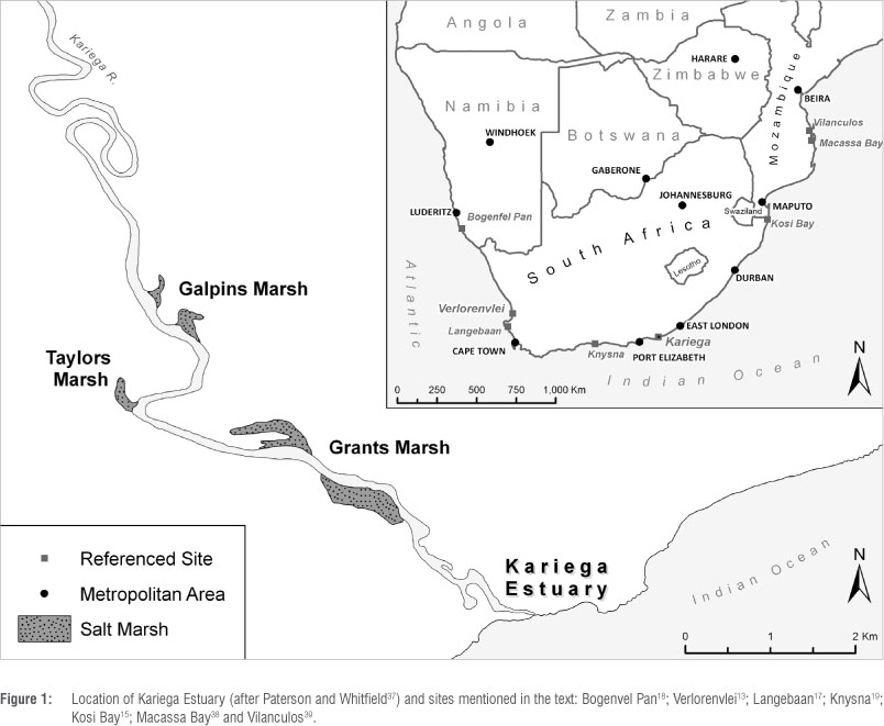
In this study we present a high-resolution foraminiferal analysis of a sedimentary sequence derived from the Kariega Estuary, Eastern Cape, South Africa (Figure 1). Modern foraminiferal assemblages analysed at this site exhibit clear vertical zonation across the marsh surface. Modern assemblages were used to construct a training set of foraminifera suitable for transfer function purposes which could then be applied to downcore fossilised assemblages. A late Holocene sea-level reconstruction chronologically controlled by accelerator mass spectrometry (AMS) radiocarbon dating is presented, representing the first high-resolution, continuous record of sea-level history for eastern South Africa.
Study site
The Kariega River is elongated and sinuous, with the estuary stretching approximately 18 km inland from the mouth (Figure 1). The estuary is surrounded by salt marshes, sand flats and steep slopes in the upper reaches.34 The system is hypersaline owing to a lack of freshwater input34; however, scouring by tidal currents maintains a permanent connection with the sea.35 As with many estuarine systems along the Eastern Cape shoreline, Kariega has a small tidal prism, with water levels fluctuating in response to semi-diurnal and spring/neap tidal cycles.36 This system has a low turbidity, with little salinity and thermal stratification of the water column during any stage of the tidal cycle.36 The system receives variable rainfall, has a small catchment area (686 km2) and is regulated by three dams.
There are three major intertidal salt-marsh systems at Kariega: Taylors, Grants and Galpins. The intertidal creeks of Taylors and Grants marshes are relatively shallow with a narrow intertidal area, while Galpins marsh- is wider and more extensive.37,40 Several characteristics of Galpins salt marsh make it an ideal location for foraminiferal analysis: (1) the marsh is attached to a small estuarine embayment, and is thus protected from erosional dynamics associated with the main channel; (2) the intertidal zone exhibits clear vegetation zonation, dominated by Spartina marítima and Sarcocorniaperennis; and (3) analysis of surface samples across the intertidal zone indicate clear vertical zonation in modern foraminiferal assemblages.
Methods
An extensive programme of coring using a 20-mm diameter gouge auger was conducted to establish the stratigraphy of the salt marsh. Core lithologies were described using notation developed by Long et al.41, based on original classification techniques by Troels-Smith43. A master core was taken from the high marsh (near the level of mean high water spring tides) for palaeoenvironmental analyses. Five neighbouring, stratigraphically consistent 1-m continuous sediment cores (KAR1-5) were extracted from this point in the salt marsh (33°39'04"S; 26°39'74"e) using a 50-mm diameter gouge auger. Cores were placed into polyvinyl chloride piping, wrapped in polythene sheeting and heavy duty plastic and transported to the laboratory for cold storage and analysis. Of the five cores, one was selected for foraminiferal analysis (KAR2) and another for developing a chronology (KAR4). Remaining cores are in cold storage for potential future studies.
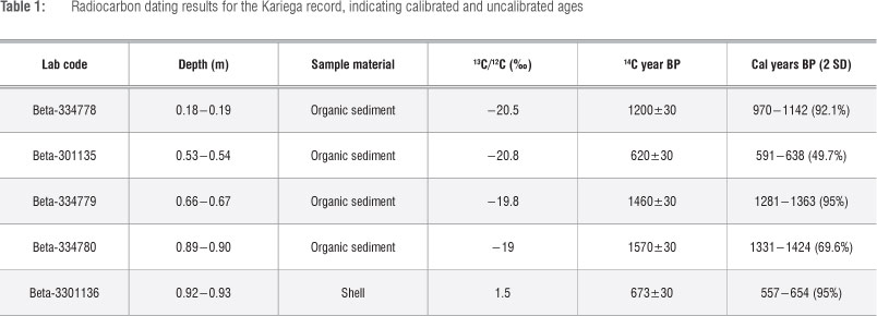
Stratigraphic boundaries were targeted for dating to produce a late Holocene chronology. Five samples were extracted from core KAR4 for AMS radiocarbon analysis at Beta Analytic (USA). The organic fraction was dated for four bulk sediment samples and the carbonate fraction for a single shell sample at the base of the core. AMS ages for bulk sediment samples were calibrated using the calibration curve SHCal04.43
The marine shell-derived age was corrected using a AR value of 146±85.44 This correction provided a spuriously young age, possibly as a result of shell recrystallisation. Several linear age modelling scenarios were considered, including the less parsimonious possibility that the shell age is correct and that overlying bulk sediment ages are all too old. In accordance with the principle of parsimony, the shell age was ultimately excluded and an objective Bayesian age-modelling exercise was applied to the remaining dates. An alternative explanation is that older sediments could have been washed downstream and deposited in the salt marsh. However, the consistently organic stratigraphy does not provide supporting evidence of sedimentary inwash events, as it lacks coarse sand layers. The majority of foraminiferal tests encountered were intact without etching, which does not support sediment reworking.
'Bacon' source code,45 within the R open-source statistical environment,46 was used to develop an age-depth model. Bacon utilises a Bayesian approach towards chronology building, which is reliant on a priori information. A mean accumulation rate of 16 cm/year was used for the model (acc.mean=16, acc.shape=2). However, as salt marsh sedimentation rates are highly variable, a low memory component was used (mem.mean=0.3, mem.strength=10). The resultant age-depth model provided age ranges at a resolution of 10-mm within 95% confidence limits. It is understood that, through using an age-depth modelling approach rather than individually dated sea-level index points, sea-level reconstruction interpretation can be compromised.8 In this instance, however, the use of Bacon facilitates the construction of a chronologically constrained sea-level history which would not be possible without age-depth modelling.
Core KAR2 was subsampled at a 20-mm downcore resolution yielding 48 samples for foraminiferal analysis following Scott and Medioli21 and Gehrels47. Samples were stored in ethanol, rinsed in distilled water and washed through 63-µm and 500-µm sieves. The larger sieve was used to remove organic matter and coarse detritus; remaining sediment on the smaller sieve was subdivided into eight aliquots using a volumetric wet splitter and retained for foraminiferal analysis. Samples were kept wet throughout the counting process to prevent aggregation of organic particles and to minimise degradation.
A Leica M205C stereomicroscope with an attached DFC295 digital camera (SMM Instruments, Durban, South Africa) was used for counting and identifying foraminiferal assemblages under 60X, 80X and 100X magnification. At least 250 individuals were counted per sample48; this limit was most necessary where indicator species were present in low numbers.47 Downcore fluctuations in foraminiferal assemblages were plotted using Psimpoll Version 4.26349; the constrained incremental sum of squares (CONISS)50 stratigraphically constrained ordination- technique assisted in defining zonation patterns of downcore fossil-ised assemblages.
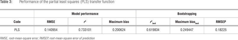
Detrended canonical correspondence analysis was used to determine the environmental (in this case elevation) gradient length of the modern foraminiferal data set in standard deviation (SD) units. Where gradient lengths are < 2 SD units, it is assumed species are responding linearly to the environmental variable.51 The data set demonstrated a short gradient length of 1.4 SD units and therefore a linear-based regression model was suitable for developing a transfer function.52 The transfer function was built using a partial least squares regression model in C253 and the modern foraminifera counts of both live and dead assemblages were combined. Training sets composed of total assemblages are still occasionally used based on the assumption that the live assemblages will in time contribute to the fossil record54; however, it is acknowledged that there are strong arguments suggesting that the dead assemblage alone is most suitable for transfer function purposes (for example, Murray55). Sample-specific elevation prediction errors were calculated using bootstrapped cross validation which provided root-mean-square error of prediction values for each fossil sample. Fossil samples that were similar in composition to the training set samples were included in the reconstruction. The modern analogue technique was used to assign a minimum dissimilarity coefficient value to all fossil samples. Similarity cut-off values follow Watcham et al.56 Samples below 0.66 m had poor fits with their closest modern analogues. These samples were manually assigned an indicative meaning associated with minimum sea-level heights only. Reconstructed elevation values for all samples were used to calculate past sea-surface elevations in relation to present MSL following Gehrels57.
Results
Stratigraphy and chronology
The basal unit for this core (0.97-0.57 m) comprises clay, silt and sand in approximately equal quantities. At around 0.92 m, a few unidentifiable shell fragments were recovered. A clay unit containing some silt is present from 0.57 m to 0.37 m. Above this unit is a clayey, silty sand lens, which is 0.70 m thick. From 0.30 m up, the lithostratigraphy is characterised by decreasing grain size (increasing clay content) and becomes increasingly organic. Between 0.70 m and the surface, there is abundant in-situ decaying organic material. Iron oxide staining is present between 0.26 m and 0.70 m.
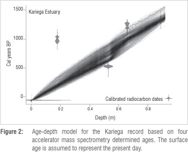
Accelerator mass spectrometry radiocarbon age determinations and their calibrated ages (with standard deviations) are presented in Table 1. The age-depth model created using Bacon is presented in Figure 2, and places the record within the late Holocene period. The basal date provides an age of 1331 to 1424 cal years BP at 0.895 m. The age determination at 0.185 m (970 to 1142 cal years BP) is identified by the model as a possible outlier.
Foraminiferal data
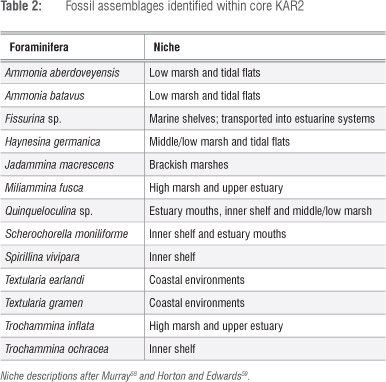
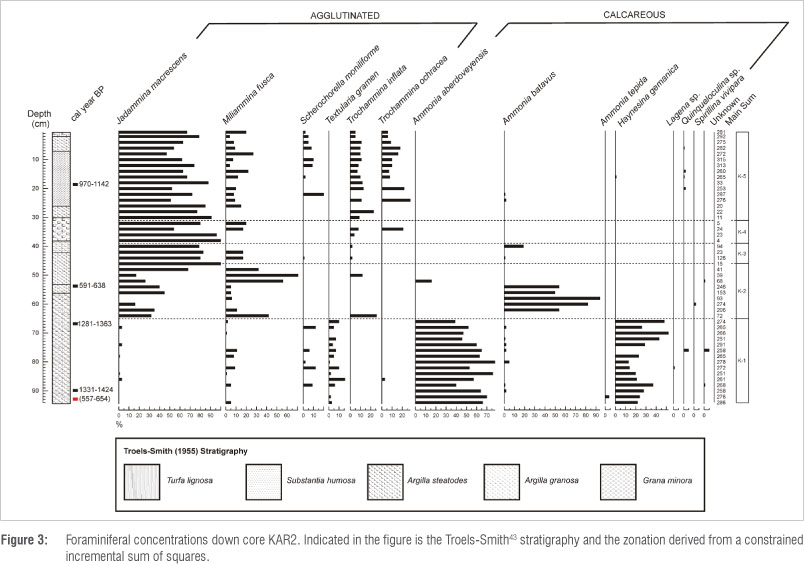
Foraminifera are present and well preserved throughout the length of the core. The majority of tests identified and counted were intact, with little evidence of corrosion. A total of 16 species were identified; the main species, alongside their common environmental niches, are presented in Table 2. Low concentrations of foraminiferal tests (<100) are present between 0.38 m and 0.26 m. Average foraminiferal test concentration for the core was 213 tests.cm3. CONISS cluster analysis identified five assemblage zones:, K-1 (0.94-0.65 m), K-2 (0.65-0.46 m), K-3 (0.46-0.39 m), K-4 (0.39-0.31 m) and K-5 (0.31-0 m). These zones differentiated major changes in foraminiferal populations through the core. Agglutinated foraminifera are most abundant in the upper reaches of the core and gradually decrease down the core, whereas the base of the core is dominated by calcareous foraminifera (Figure 3).
Zone K-1 at the base of the core is dominated by the calcareous species Ammonia aberdoveyensis and Haynesina germanica, which commonly comprise up to 90% of the assemblage. At 0.66 m there is a shift away from these species towards Ammonia batavus and the agglutinated salt-marsh species Jadammina macrescens and Miliammina fusca (Zone K-2). J. macrescens is the most abundant species in Zone K-3 which includes low numbers of M. fusca and Trochammina inflata. Zones K-4 and K-5 are dominated by J. macrescens. From Zone K-4 upwards there is an increasing diversity of agglutinated foraminiferal species. T. inflata and Trochammina ochracea represent up to 40% of the assemblage in Zone K-5.
Quantitative reconstruction
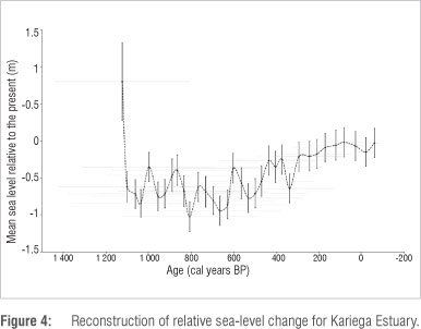
Indicative-meaning based predictions of palaeomarsh-surface elevations were converted into sea-level estimates following Gehrels57. Samples with good or close modern analogue fits were reconstructed using the transfer function (Table 3). Those samples with poor fit represent foraminiferal assemblages which had no close modern analogues from the training set (Table 4). The presence of H. germanica in these samples was used to provide a sea-level estimate. This species most commonly occupies the intertidal zone61 and therefore an indicative range from- lowest astronomical tide (-1.04 m above MSL) to the lowermost sample from the training set (0.01 m above MSL) was applied to these samples. Each sample was constrained chronologically using interpolated values from the age-depth model. The reconstructed sea-level curve for Kariega Estuary (Figure 4) identifies rapid RSL fall at around 1100 cal years BP to levels down to a minimum of ~1 m below present MSL. Between 1100 and 300 cal years BP, RSL appeared to fluctuate at approximately 150-year periods, with amplitudes of around 0.5 m. After 300 cal years BP RSL remained relatively stable.
Discussion
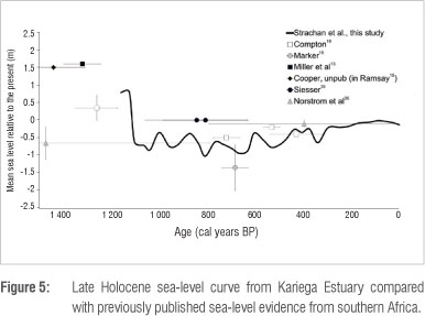
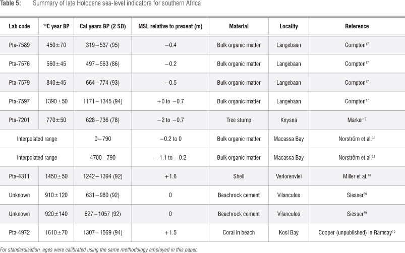
The Kariega Estuary appears to have been connected to the open ocean throughout the late Holocene, based on continuous foraminiferal presence throughout the core. The fossil microfauna suggest that prior to 1100 cal years BP RSL was higher than it is today, in accordance with existing literature.13,16,17 The calcareous foraminiferal assemblages from the lowest ~0.35 m of the core imply the existence of a low intertidal, or possibly shallow subtidal, environment before 1100 cal years BP Because of the broad habitual range of calcareous foraminifera, it is difficult to determine precise indicative meanings from these assemblages.25,48 Despite this difficulty, it is clear that the reconstruction encompasses the falling limb of rapid RSL decline out of the late Holocene highstand which is documented across South African coastlines.17,19 Existing late Holocene sea-level data from South Africa is summarised in Table 5 and presented alongside the modelled reconstruction (Figure 5). There is strong agreement between the existing data and the RSL curve from the-Kariega Estuary which provides a well vertically constrained estimate of continuous late Holocene RSL for this part of Africa.
Pre-1100 cal years BP highstand
A late Holocene sea-level highstand has been reported at around 1500-1200 cal years BP13,15,17 (Figure 5). A sea-level curve from the southwestern coast,18 and to some extent beachrock evidence from the KwaZulu-Natal coast,14 indicate highstands between 3000 and 1200 cal years BP The Zostera facies recovered from Langebaan,17 a pollen record from Verlorenvlei16 and oyster shells from Langebaan61 present further evidence that RSL was 0.5-0.7 m higher than present at around 1300 cal years BP. This highstand corresponds with the Little Climatic Optimum, a period of temperate warming which is associated with higher sea levels around this time.62 The RSL decline out of this highstand is identified by significant changes in foraminiferal assemblages from Kariega. As RSL fell below that of modern day, the abrupt change in foraminifera populations at 0.66 m might be a result of sedimentary erosion as sea levels began to rise out of the lowstand. High precision dating would be required to determine whether a hiatus exists at this level.
1100-300 cal years BP oscillations
The Kariega record provides evidence of sea levels remaining lower (by approximately 0.5 m) than present MSL from ~1100 to ~300 cal years BP Siesser's39 study at Vilanculos, using beachrock cement, suggests that sea levels were equivalent to the present day from 842±215 cal years BP (Figure 5), contradicting other studies which indicate a lower RSL during this period. According to Compton17, two lowstands of -0.5 m to -1 m took place from 700 to 400 cal years BP (Figure 5). This lowstand is evident on the south coast at 682 ± 54 cal years BP from in-situ tree stumps exposed at Knysna Estuary during low tide19 (Figure 5). This lowstand corresponds with lower sea-surface temperatures between 500 and 400 cal years BP; therefore steric effects associated with cool water temperatures may have been a contributing factor.17
300 cal years BP to present
The RSL oscillations shown by this study and by Compton17 terminate at around 300 cal years BP. Following 300 cal years BP, RSL shows a gradual rise to present MSL. Evidence from Langebaan Lagoon17 (Figure 5) suggests that sea level has been rising to present levels since 400 cal years BP. The Kariega reconstruction shows relatively stable sea levels throughout the past 300 cal years BP. Exogenic subsidence linked with large-scale water extraction would likely result in recent (past 100 years) sea-level rise. Such evidence is absent from the Kariega reconstruction, suggesting that local subsidence has not occurred.
The Macassa Bay study indicates that lower sea levels are followed by a rise from 700 cal years BP until the present38 (Figure 5). However, this multi-proxy data set implies that relatively low sea levels recorded at Macassa Bay were associated with a freshwater phase with little influence from marine processes.38 A noticeable sea-level acceleration occurs in the RSL reconstruction during the middle of the 20th century following a minor RSL fall during the early 1900s. This pattern of recent sea-level change has also been documented in New Zealand and Tasmania.12 Such similarities with other southern hemispheric RSL curves lend weight to the credibility of this study. Proposed sources for this 20th-century sea-level inflexion include northern hemispheric ice melt from Greenland.12
The Kariega record provides high-resolution sea-level data at a regional scale, offering insight into east coast sea-level fluctuations. The pre-1100 cal years BP highstand is supported by existing sea-level data, which provide good chronological estimation of when RSL declined out of this highstand. Observed fluctuations during the late Holocene have been small (~ 0.5 m amplitude) compared with the mid-Holocene (~2-3.5 m amplitude15). Reconstructed patterns of recent RSL changes are in agreement with other records from the southern hemisphere, reflecting processes contributing to sea-level change occurring on hemispheric, or greater, scales.
Few tidal gauge records for the southern hemisphere extend beyond 50 years.22 This lack of long-term tidal gauge data hampers detailed validation of recent reconstructions. To identify and understand patterns of both recent (i.e. 19th and 20th century) and late Holocene sea-level changes, it is necessary to consider proxy data.1,7 Further research sites should be investigated along the east coast to establish a greater modern-day analogue for South Africa and to strengthen future reconstructions. Sea-level reconstructions from neighbouring sites could present a more robust and high-resolution picture of sea-level fluctuations for the east coast of South Africa.
Conclusion
Fossil foraminiferal assemblages analysed from a ~1200-year sedimentary record from the Kariega Estuary, South Africa, identify continuous late Holocene RSL changes that show accordance with published records. The reconstruction was supported chronologically using a Bayesian age-depth model based on AMS radiocarbon- age determinations. With higher resolution dating, timings of key RSL changes in South Africa could be established with previously unprecedented accuracy. This study presents the first salt-marsh foraminifera transfer function for the southern African coastline used to produce a high-resolution sea-level curve for the Kariega Estuary. A late Holocene RSL was reconstructed with mean errors of ±0.2 m. A sea-level highstand was dated to pre-1100 cal years BP. We observed fluctuations in MSL between 1100 and 300 cal years BP; yet MSL then was consistently lower than present sea levels. From 300 cal years BP, RSL increased gradually to present-day levels, and a sea-level inflexion was shown to occur at some time during the mid-20th century. The results of this study suggest that intertidal salt-marsh foraminifera demonstrate potential for high-resolution reconstruction of RSL change in South Africa.
Acknowledgements
This research was financially supported by the National Research Foundation. Angus Paterson (SAEON) facilitated access to the study site. Martin Hill and Julie Coetzee (Rhodes University) assisted in fieldwork. Jussi Baade (University of Jena) assisted with GPS data. Brice Gijsbertsen (UKZN) professionally drafted Figure 1.
Authors' contributions
All authors contributed equally to the project conceptualisation, fieldwork and write-up. K.L.S. performed the laboratory and microscopy analyses.
References
1. Douglas BC. Concerning evidence for fingerprints of glacial melting. J Coast Res. 2008;24:218-227. http://dx.doi.org/10.2112/06-0748.1 [ Links ]
2. Nerem RS. Measuring global mean sea level variations using TOPEX/ POSEIDON altimeter data. J Geophys Res. 1995;100(25):135-151. [ Links ]
3. Gehrels R, Horton BP Kemp AC, Sivan D. Two millennia of sea-level data: The key to predicting change. EOS Trans Am Geophys Union. 2011;92(35):289-296. http://dx.doi.org/10.1029/2011EO350001 [ Links ]
4. Cronin TM. Rapid sea-level rise. Quat Sci Rev. 2012;56:11-30. http://dx.doi.org/10.1016/j.quascirev.2012.08.021 [ Links ]
5. Church JA, White NJ. Sea-level rise from the late 19th to early 21st century. Surv Geophys. 2011;32:585-602. http://dx.doi.org/10.1007/s10712-011-9119-1 [ Links ]
6. Nicholls RJ, Marinova N, Lowe JA, Brown S, Vellinga P De Gusmae D, et al. Sea-level rise and its possible impacts given a 'beyond 4°C world' in the twenty-first century. Philos Trans R Soc Lond A. 2011;369:161-181. http://dx.doi.org/10.1098/rsta.2010.0291 [ Links ]
7. Siddall M, Milne GA. Understanding sea-level change is impossible without both insights from paleo studies and working across disciplines. Earth Planet Sci Lett. 2012;315-316:2-3. http://dx.doi.org/10.1016/j.epsl.2011.10.023 [ Links ]
8. Gehrels WR, Woodworth PL. When did modern rates of sea-level rise start? Global Planet Change. 2013;100:263-277. http://dx.doi.org/10.1016/j.gloplacha.2012.10.020 [ Links ]
9. Pirazzoli PA, Pluet J. World atlas of Holocene sea-level changes. Amsterdam: Elsevier; 1991. [ Links ]
10. Goodwin IAND. Did changes in Antarctic ice volume influence late Holocene sea-level lowering? Quat Sci Rev. 1998;17:319-332. http://dx.doi.org/10.1016/S0277-3791(97)00051-6 [ Links ]
11. Gehrels WR, Hayward BW, Newnham RM, Southall KE. A 20th century acceleration of sea-level rise in New Zealand. Geophys Res Lett. 2008;35:1-5. http://dx.doi.org/10.1029/2007GL032632 [ Links ]
12. Gehrels WR, Callard SL, Moss PT, Marshall WA, Blaauw M, Hunter L, et al. Nineteenth and twentieth century sea-level changes in Tasmania and New Zealand. Earth Planet Sci Lett. 2012;315-316:94-102. http://dx.doi.org/10.1016/j.epsl.2011.08.046 [ Links ]
13. Miller D, Yates R, Jerardino A, Parkington J. Late Holocene coastal change in the southwestern Cape, South Africa. Quat Int. 1995;29:3-10. http://dx.doi.org/10.1016/1040-6182(95)00002-Z [ Links ]
14. Ramsay PJ, Cooper JAG. Late Quaternary sea-level change in South Africa. Quat Res. 2002;57:82-90. http://dx.doi.org/10.1006/qres.2001.2290 [ Links ]
15. Ramsay P. 9000 years of sea-level change along the southern African coastline. Quat Int. 1995;31:71-75. http://dx.doi.org/10.1016/1040-6182(95)00040-P [ Links ]
16. Baxter AJ, Meadows ME. Evidence for Holocene sea-level change at Verlorenvlei, Western Cape, South Africa. Quat Int. 1999;56:65-79. http://dx.doi.org/10.1016/S1040-6182(98)00019-6 [ Links ]
17. Compton JS. Holocene sea-level fluctuations inferred from the evolution of depositional environments of southern Langebaan Lagoon salt marsh, South Africa. Holocene. 2001;11:395-405. http://dx.doi.org/10.1191/095968301678302832 [ Links ]
18. Compton JS. The mid-Holocene sea-level highstand at Bogenfels Pan on the southwest coast of Namibia. Quat Res. 2006;66:303-310. http://dx.doi.org/10.1016/j.yqres.2006.05.002 [ Links ]
19. Marker ME. Evidence for a Holocene low sea level at Knysna. S Afr Geogr J (Special Edition). 1997;79(2):106-107. http://dx.doi.org/10.1080/0373624 5.1997.9713631 [ Links ]
20. Scott DB, Medioli FS. Vertical zonations of marsh foraminifera as accurate indicators of former sea levels. Nature. 1978;272:528-531. http://dx.doi.org/10.1038/272528a0 [ Links ]
21. Scott DB, Medioli FS. Quantitative studies of marsh foraminifera distributions in Nova Scotia: Implications for sea level studies. Cushman Foundation for Foraminiferal Research Special Publication. 1980;17:58. [ Links ]
22. Massey AC, Gehrels WR, Charman DJ, White SV. An intertidal foraminifera-based transfer function for reconstructing Holocene sea-level change in Southwest England. J Foramin Res. 2006;36(3):215-232. http://dx.doi.org/10.2113/gsjfr.36.3.215 [ Links ]
23. Leorri E, Gehrels WR, Horton BP, Fatela F, Cearreta A. Distribution of foraminifera salt marshes along the Atlantic coast of SW Europe: Tools to reconstruct past sea-level variations. Quat Int. 2010;221:104-115. http://dx.doi.org/10.1016/j.quaint.2009.10.033 [ Links ]
24. Gehrels WR. Determining relative sea-level change from salt-marsh foraminifera and plant zones on the coast of Maine, USA. J Coast Res. 1994;10(4):990-1009. [ Links ]
25. Woodroffe SA, Horton BP, Larcombe P. Whittaker JE. Intertidal mangrove foraminifera from the central Great Barrier Reef shelf, Australia: Implications for sea-level reconstruction. J Foramin Res. 2005;35(3):259-270. http://dx.doi.org/10.2113/35.3.259 [ Links ]
26. McMillan IK. Foraminiferal biostratigraphy, sequence stratigraphy and interpreted chronostratigraphy of marine Quaternary sedimentation on the South African continental shelf. S Afr J Sci. 1993;89:83-89. [ Links ]
27. McMillan IK. Cainozoic planktonic and larger foraminifera distributions around southern Africa and their implications for past changes of oceanic water temperatures. S Afr J Sci. 1986;82:66-69. [ Links ]
28. Cooper JAG, McMillan IK. Foraminifera of the Umgeni Estuary, Durban and their sedimentological significance. S Afr J Geol. 1987;90(4):489-498. [ Links ]
29. McMillan IK. Foraminifera from the Late Pleistocene (Latest Eemian to Earliest Weichselian) Shelly Sands of Cape Town City Centre, South Africa. Ann S Afr Mus. 1990;99(5):121-186. [ Links ]
30. Lindsay P Pillay S, Wright CI, Manson TR. Sedimentology and dynamics of the Mfolozi Estuary, north KwaZulu-Natal, South Africa. S Afr J Geol. 1996;99:327-336. [ Links ]
31. Wright CI, McMillan IK, Mason TR. Foraminifera and sedimentation patterns in St. Lucia Estuary mouth, Zululand, South Africa. S Afr J Geol. 1990;93(4):592-601. [ Links ]
32. Martin RA. Benthic foraminifera from the Orange-Luderitz shelf, southern continental margin. Joint Geological Survey/University of Cape Town Marine Geoscience Group Bulletin. 1981;11:75. [ Links ]
33. Franceschini G, McMillan IK, Compton JS. Foraminifera of Langebaan Lagoon salt marsh and their application to the interpretation of late Pleistocene depositional environments at Monwabisi, False Bay coast, South Africa. S Afr J Geol. 2005;108:285. http://dx.doi.org/10.2113/108.2.285 [ Links ]
34. Grange N, Whitfield AK, De Villiers CJ, Allanson BR. The response of two South African east coast estuaries to altered river flow regimes. Aquat Conserv. 2000;10:155-177. http://dx.doi.org/10.1002/1099-0755(200005/06)10:3< 155::AID-AQC406>3.0.CO;2-Z [ Links ]
35. Paterson AW, Vorwerk PD, Froneman PW, Strydom NA, Whitfields AK. Biological responses to a resumption in river flow in a freshwater deprived, permanently open southern African estuary. Water SA. 2008;34(5):597-604. [ Links ]
36. Taylor DI. Tidal exchange of carbon, nitrogen and phosphorus between a Sarcocornia salt marsh and the Kariega estuary, and the role of salt marsh brachyuran in this transfer [thesis]. Grahamstown: Rhodes University; 1987. [ Links ]
37. Paterson AW, Whitfield AK. Do shallow-water habitats function as refugia for juvenile fishes? Est Coast Shelf Sci. 2000;51:359-364. http://dx.doi.org/10.1006/ecss.2000.0640 [ Links ]
38. Nõrstrom E, Risberg J, Grondahl H, Holmgren K, Snowball I, Mugabe JA, et al. Coastal paleo-environment and sea-level change at Macassa Bay, south Mozambique, since c 6600 cal BP. Quat Int. 2012;260:153-163. http://dx.doi.org/10.1016/j.quaint.2011.11.032 [ Links ]
39. Siesser WG. Relict and recent beachrock from southern Africa. Geol Soc Am Bull. 1974;85:1849-1854. http://dx.doi.org/10.1130/0016-7606(1974)85<1849:RARBFS>2.0.CO;2 [ Links ]
40. Paterson AW, Whitfield AK. The ichthyofauna associated with an intertidal creek adjacent eelgrass beds in the Kariega Estuary, South Africa. Environ Biol Fish. 2000;58:154-156. http://dx.doi.org/10.1023/A:1007629328937 [ Links ]
41. Long AJ, Innes JB, Shennan I, Tooley MJ. Coastal stratigraphy: A case study from Johns River, Washington, USA. In: Jones AP, Tucker ME, Hart JK, editors. The description and analysis of Quaternary stratigraphic field sections. Technical Guide No 7. London: Quaternary Research Association; 1999. p. 267-286. [ Links ]
42. Troels-Smith J. Characterization of unconsolidated sediments. D.G.U. IV Rekke. 1955;3(10):37-82. [ Links ]
43. McCormac FG, Hogg AG, Blackwell PG, Buck CE, Higham TFG, Reimer PJ. SHCal04 southern hemisphere calibration, 0-11.0 cal years BP Radiocarbon. 2004;46:1087-1092. [ Links ]
44. Dewar G, Reamer PJ, Sealy J, Woodborne S. Holocene marine radiocarbon reservoir correction (AR) for the west coast of South Africa. Holocene. 2012;22(12):1438-1446. http://dx.doi.org/10.1177/0959683612449755 [ Links ]
45. Blaauw M, Christen JA. Flexible paleoclimate age-depth models using an autoregressive gamma process. Bayesian Anal. 2011;6(3):457-474. http:// dx.doi.org/10.1214/ba/1339616472 [ Links ]
46. Team RDC. A language and environment for statistical computing. Vienna: R Foundation for Statistical Computing; 2010. Available from: http://www.R-project.org. [ Links ]
47. Gehrels WR. Intertidal foraminifera as palaeoenvironmental indicators. In: Haslett SK, editor. Quaternary environmental micropalaeontology. London: Oxford University Press; 2002. [ Links ]
48. Horton BP Murray JW. The roles of elevation and salinity as primary controls on living foraminiferal distributions: Cowpen Marsh, Tees Estuary, UK. Mar Micropaleontol. 2007;63:169-186. http://dx.doi.org/10.1016/j.marmicro.2006.11.006 [ Links ]
49. Bennett KD. Psimpoll: C programs for plotting pollen diagrams and analysing pollen data. Villavgen: Uppsala Universitet; 2005. [ Links ]
50. Grimm EC. CONISS: A FORTRAN 77 program for stratigraphically constrained cluster analysis by the method of incremental sum of squares. Comput Geosci.1987;13:13-35. http://dx.doi.org/10.1016/0098-3004(87)90022-7 [ Links ]
51. Ter Braak CJF, Prentice IC. A theory of gradient analysis. Adv Ecol Res. 1988;18:271-317. http://dx.doi.org/10.1016/S0065-2504(08)60183-X [ Links ]
52. Birks HJB. Quantitative palaeoenvironmental reconstructions. In: Maddy D, Brew JS, editors. Statistical modeling of Quaternary science data. Technical Guide No 5. Cambridge: Quaternary Research Association; 1995.p. 161-236. [ Links ]
53. Juggins S. C2 Version 1.3: Software for ecological and palaeoecological data analysis and visualization. Newcastle upon Tyne: Department of Geography, University of Newcastle; 2003. p. 69. [ Links ]
54. Booth RK, Lamentowicz M, Charman DJ. Preparation and analysis of testate amoebae in peatland palaeoenvironmental studies. Mires Peat. 2010;7:1-7. [ Links ]
55. Murray JW. The enigma of the continued use of total assemblages in ecological studies of benthic foraminifera. J Foramin Res. 2000;30(3):244-245. http://dx.doi.org/10.2113/0300244 [ Links ]
56. Watcham EP Shennan I, Barlow NLM. Scale considerations in using diatoms as indicators of sea-level change: Lessons from Alaska. J Quaternary Sci. 2013;28(2):165-179. http://dx.doi.org/10.1002/jqs.2592 [ Links ]
57. Gehrels WR. Middle and late Holocene sea-level changes in eastern Maine reconstructed from foraminiferal salt marsh stratigraphy and AMS 14C dates on basal peat. Quat Res. 1999;52:350-359. http://dx.doi.org/10.1006/qres.1999.2076 [ Links ]
58. Murray JW. British near shore foraminiferids: Key and notes for the identification of the species. London: Academic Press; 1979. [ Links ]
59. Horton BP, Edwards RJ. Quantifying Holocene sea-level change using intertidal foraminifera: Lessons from the British. Cushman Foundation for Foraminiferal Research Special Publication. 2006;40:97. [ Links ]
60. Murray JW. Ecology and application of benthic foraminifera. Cambridge: Cambridge University Press; 2006. [ Links ]
61. Flemming BW. Depositional processes in Saldanha Bay and Langebaan Lagoon. Marine Geoscience Bulletin. 1997;8:215. [ Links ]
62. Nunn PD. Sea-level changes over the past 1000 years in the Pacific. J Coast Res. 1998;14:23-30. [ Links ]
 Correspondence:
Kate Strachan
Discipline of Geography, School of Agricultural, Earth & Environmental Sciences
University of KwaZulu-Natal
Private Bag X01, Scottsville 3201, South Africa
email: kateleighstrachan@gmail.com
Received: 25 Jun. 2013
Revised: 07 Oct. 2013
Accepted: 12 Oct. 2013
© 2014. The Authors. Published under a Creative Commons Attribution Licence.

