RESEARCH LETTER

 

Mid-latitude ionospheric signature of a weak solar flare in winter

 

 

Etienne J. Koen^{I, II}; Andrew B. Collier^{I, III}

^ISANSA Space Science, Hermanus, South Africa
^IISpace and Plasma Physics, Royal Institute of Technology, Stockholm, Sweden
^IIISchool of Chemistry, University of KwaZulu-Natal, Durban, South Africa

Correspondence to

 

 

---

ABSTRACT

Measurements of the amplitude and phase of very low frequency transmitter signals were used to evaluate the effects on the ionosphere of a moderate intensity solar flare that occurred on 13 December 2007. These measurements were compared to modelled results from the Long Wave Propagation Capability code. The ionospheric effects were found to be delayed by ~1 min with respect to the 0.1-0.8 nm solar X-ray flux.

Keywords: VLF; solar flare; D-region; ionosphere; X-ray

---

 

 

Introduction

Waveguide propagation

Very low frequency (VLF) radio waves span the frequency interval 3-30 kHz. The surface of the Earth is a good conductor at VLF, especially over the oceans. The ionosphere also represents a conducting surface for VLF waves. The cavity between these two conducting surfaces forms the Earth-ionosphere waveguide (EIWG), in which VLF waves may propagate enormous distances while experiencing minimal attenuation (about 1.5 dB/Mm). Although the characteristics of the Earth are relatively constant, the ionosphere is dynamic over a range of time scales. As a result of changes in incident solar UV radiation, the density of the ionosphere exhibits a regular diurnal variation. The passage of the seasons also has an impact on local ionospheric characteristics. Both of these variations are stable and predictable. Unpredictable phenomena, such as particle precipitation from the radiation belts and solar flares, also influence the ionosphere.

The D-region

The D-region (about 60-90 km above the Earth's surface) is the lowest part of the ionosphere and is maintained during the day mainly by Lyman- α radiation from the sun which ionises nitric oxide.¹ It is convenient to characterise the D-region by a height-dependent conductivity²:

where ω₀( s^-1) is the electron plasma frequency and v is the effective electron-neutral collision frequency. The profile is determined by the sharpness parameter β (in km^-1) and the reflection height H' (in km). The electron density profile associated with Equation 1 increases exponentially with height³:

where

Solar flares

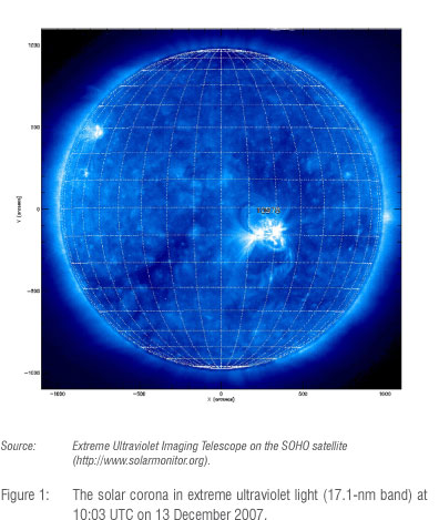
Solar flares are violent explosions in the sun's chromosphere which release a huge number of energetic particles and are accompanied by a rapid and intense increase in brightness. Solar flares produce radiation which spans the entire electromagnetic spectrum from radio waves to gamma rays. Most flares occur in active regions around sunspots, where magnetic fields penetrate the photosphere to link the corona to the solar interior. In most cases solar flares are accompanied by coronal mass ejections but there is not necessarily a causal link. Figure 1 depicts an image of the C4.5 solar flare that occurred on 13 December 2007.

 

 

Under normal conditions, the solar X-ray flux is too small to be a significant source of ionisation in the D-region. However, during a solar flare, X-rays with wavelengths appreciably below 1 nm are able to penetrate down to the D-region, causing additional ionisation of all atmospheric constituents, including N₂ and O₂. The enhanced ionisation is reflected by a decrease in H and an increase in β.

Relationship between X-ray flux and VLF signal

Only the illuminated portion of propagation paths in the EIWG were considered because X-rays take about 8 min to arrive at the Earth and the ionising effects of a solar flare are thus almost immediate. The enhanced ionisation decays slightly more slowly than the X-ray flux and the ionospheric effects do not last long enough to be evident on the night side of the propagation paths.

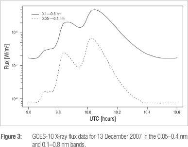
The satellites of the Geostationary Operational Environmental Satellite (GOES) system record X-fluxes in the 0.050.4 nm and 0.1-0.8 nm bands. These data are routinely used to monitor solar flares. The enhanced ionisation generated by solar flare X-rays lowers the reflection height of the ionosphere, thereby affecting signals propagating in the EIWG. The signal amplitude can increase or decrease, depending on the interference conditions and the creation of new modes. The magnitude of these effects depends on the intensity of the X-ray flux. The signal phase is also affected and the phase change has been found to be nearly proportional to the logarithm of the X-ray flux.⁴ This proportionality was used to determine the class of the solar flare which occurred on 04 November 2003 - the strongest flare ever detected by the GOES satellites.^5,6 This flare could not be classified because the X-ray detector on GOES was saturated. Here, we present the effects of a flare of class C4.5 which occurred on 13 December 2007; although relatively weak, this flare is interesting in that it had two intensity peaks.

Long Wave Propagation Capability code

The theory of VLF propagation in the EIWG is well established for quiet ionospheric conditions. A series of computer programs has been developed by the Naval Ocean Systems Center (San Diego, USA) to predict the change in VLF amplitude and phase along a transmission path. The Long Wave Propagation Capability (LWPC) code is part of this series.⁷ The model specified in LWPC has an ionosphere which is described by Equation 2. This equation enables one to infer Wait's parameters, H and β, from measurements of VLF propagation.

In its simplest form, LWPC is used to calculate the amplitude and phase versus distance from the transmitter for given ground and ionospheric conductivities. The ground conductivity parameters are constant in time. The ionospheric conditions vary along a transmission path depending on the local solar zenith angle. One limitation of LWPC is that it does not take into consideration the effects of solar activity on the ionosphere. However, it does consider geomagnetic activity.

Together with VLF observations, LWPC was used to examine the evolution of the amplitude and phase perturbations for the entire duration of the solar flare that occurred on 13 December 2007. At the peak irradiance of the flare, the electron density profile was found by varying H and β as inputs to the LWPC code until the modelled phase and amplitude matched the observations.

 

Data

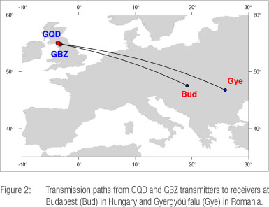
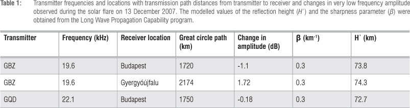
VLF transmitters are distributed at various locations across the globe; some transmitters are used by the US Navy to communicate with submarines. The transmitter signals are also recorded by narrowband VLF receivers located in several countries and used for scientific research. A list of transmitters from which data were derived in this study is given in Table 1. All the signals travelled over land from west to east. The propagation paths were reasonably stable on the dayside of the terminator passage.

VLF recordings were made at Budapest, Hungary (47°28' N, 19°03' E) and Gyergyóújfalu, Romania (46°38' N, 25°36' E). The transmission paths are shown in Figure 2. The receiver sampling rate was 12 Hz and the data was smoothed with a 5 s running mean. All phase recordings are referenced to GPS time.

 

 

Analysis and results

There were 21 solar flares with classes greater than C1 detected by the GOES satellites during the period from 14 July 2007 to 17 May 2008. Of these flares, 14 occurred on the illuminated portion of the transmission paths considered in this study. Only five of these flares produced signatures which were evident in the VLF data. The remainder of the flares occurred where the data were either too noisy or, in most cases, during the passage of the solar terminator across the transmission path.

The most intense flare occurred on 13 December 2007, which was close to solar minimum, and is classified as a C4.5 with a peak flux of 4.5 μW/ m². The flare started at 09:39 UTC and ended at 10:09 UTC; its peak intensity occurred at 10:03 UTC. The flare was observed by GOES in both the 0.05-0.4 nm and 0.1-0.8 nm X-ray bands (Figure 3). The X-ray signature had a double peak, with the second peak greater in amplitude than the first. The flare was identified on five VLF transmission paths, of which three are presented here. Examples of the VLF signatures are given in Figure 4. There was a decrease in the amplitude of the signal from the GBZ transmitter at the time of the flare (Figure 4a). The double peak is clearly visible in the phase of the signal from the GQD transmitter (Figure 4c). Amplitude perturbations were observed on signals from both the GBZ and GQD transmitters (Figures 4a and 4b).

 

 

The modelled values for H' and β were modified iteratively until the change in amplitude and phase calculated by LWPC matched the VLF observations. The unperturbed values of H and β depended on the solar zenith angle at the midpoint of each transmission path⁸ and were taken to be H' = 77.2 km and β = 0.26 km¹.

The calculated values for H' and β at the instant of peak X-ray flux are given in Table 1. H' was found to decrease by ~3.6 km and β to increase by ~0.04 km^-1. The values for GBZ differed only slightly from those for GQD, where both the amplitude and phase were recorded and H' and β were calculated simultaneously.

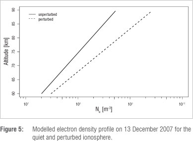
Using Equation 2, the electron density profiles were constructed for the unperturbed and perturbed conditions. Electron density in the altitude range of 60-90 km is of particular importance as it determines VLF propagation characteristics. The logarithm of the electron density versus altitude is plotted in Figure 5. The most evident effect of the solar flare was the increase in the gradient as a result of the increase in β at the time of the flare. The flare ionised the D-region down to lower altitudes, resulting in an increase in the slope of the electron density profile.

 

 

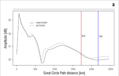
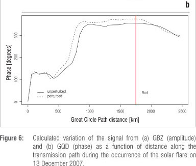
From the calculated values for H' and β the variations in amplitude and phase versus distance were calculated using LWPC and are presented in Figure 6. The vertical solid lines indicate the distances from the transmitters to the receivers. Generally, all the modal minima were found to move towards the transmitter during a flare.⁹ There are certain locations close to a modal minimum that are more sensitive to the effects of the flare, with the result that a greater variation of the signal is observed at these locations. For the GBZ transmitter (Figure 6a), the Gyergyóújfalu receiver was more sensitive to the flare than was the receiver at Budapest. The phase variation along the GQD path (Figure 6b) shows the modal minima moving towards the transmitter from 500 km to 440 km and a phase advance at the Budapest receiver.

 

 

For comparison between the X-ray flux and VLF data, the diurnal trend for each of the signals was removed. After detrending, a low pass filter was applied to the VLF data, removing variations with periods less than 400 s. This comparison is given without any time shift. The double peak of the flare is apparent in all the VLF data. The GBZ power (Figure 7a, right panel) shows a linear relationship with the 0.1-0.8 nm band X-ray flux. Comparing the same VLF data to the 0.05-0.4 nm band (Figure 7a, left panel), the VLF signal seemed to react to the X-rays with a delay and recovered more slowly.

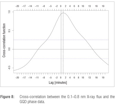
The phase of the GQD signal tracks the X-ray flux quite closely, especially up to the peak in the 0.1-0.8 nm band (Figure 7b, right panel). It appears that the phase and the X-ray flux are linearly related. The 0.05-0.4 nm band (Figure 7b, left panel) does not correlate as well, but both the phase and X-ray flux generally track up and down together. Figure 8 illustrates the cross-correlation between the VLF phase and the GOES X-ray flux, which indicates a strong correlation at a lag of 1 min.

 

 

Discussion and conclusions

A C4.5 solar flare that occurred on 13 December 2007 produced perturbations in the VLF amplitude and phase on mid-latitude subionospheric paths during winter. The reference height was found to decrease by ~3.6 km and the sharpness to increase by ~0.04 km^-1. For comparison, Zigman et al.¹⁰ (also using LWPC) showed that H' decreased by 6.6 km and β increased by ~0.11 km¹ for a C3.2 flare. The signatures of the flare appeared in the VLF data within ~1 min of the enhanced X-ray flux.

The VLF phase was found to be in closer agreement with the variations in X-ray flux data than the power. There appeared to be a linear relationship between the VLF phase and the 0.1-0.8 nm X-ray flux. These results differ from previous findings where the logarithm of the X-ray flux scaled almost linearly with the VLF phase.^4,6 While the flare investigated by McRae and Thomson⁴ had a flux of 4.5 mW/m², the one discussed here is three orders of magnitude weaker, having a flux of only 4.5 μW/m². Moreover, the flare investigated by McRae and Thomson⁴ occurred during a time close to solar maximum where the background X-ray level was observed to be above 4.2 mW/m² while the background X-ray level for the flare studied here was about 4.2 μW/m². Raulin et al.¹¹ showed that there is a solar cycle dependence in the signature of solar flares in subionospheric propagation data. The ionosphere tends to be more responsive during higher solar activity. When there is such a small range in variation, the presence of noise can make it difficult to tell whether a relationship is linear or logarithmic. However, Raulin et al.¹² reported that flares greater than C3 should be easy to resolve in the VLF data.

 

Acknowledgements

We would like to thank János Lichtenberger and Peter Steinbach of the Space Research Group, Eotvos University, Budapest for collecting the VLF data. We also thank the US Navy for the use of the LWPC program. GOES data were obtained from US National Geophysical Data Center (NGDC) at htpp://www.ngdc.noaa.gov

 

Authors' contributions

E.K. was the project leader; he performed the modelling, wrote the manuscript and produced the figures. A.C. supervised the work.

 

References

1. Banks PM, Kockarts G. Aeronomy. San Diego, CA: Academic; 1973.         [ Links ]

2. Wait JR, Spies KP Characteristics of the Earth-ionosphere waveguide for VLF radio waves. NBS technical note 300. Washington DC: US Department of Commerce, National Bureau of Standards; 1964.         [ Links ]

3. Thomson NR. Experimental daytime VLF ionospheric parameters. J Atmos Terr Phys. 1993;55:173-184. http://dx.doi.org/10.1016/0021-9169(93)90122-F        [ Links ]

4. McRae WM, Thomson NR. Solar flare induced ionospheric D-region enhancements from VLF phase and amplitude observations. J Atmos Terr Phys. 2004;66(1):77-87. http://dx.doi.org/10.1016/j.jastp.2003.09.009        [ Links ]

5. Thomson NR, Rodger CJ, Dowden RL. Ionosphere gives size of greatest solar flare. J Geophys Res. 2004;31:L06803.         [ Links ]

6. Thomson NR, Rodger CJ, Clilverd MA. Large solar flares and their ionospheric D region enhancements. J Geophys Res. 2005;110:1-10.         [ Links ]

7. Fergusson A. Computer programmes for assessment of long-wavelength radio communications. Version 2.0. Technical document 3030. San Diego, CA: Space and Naval Warfare Systems Center; 1998.         [ Links ]

8. Morfitt D. Effective electron density distributions describing VLF/ELF propagation data. Naval Ocean Systems Center Technical Report NOSC/TR 141. Springfield, VA: National Technical Information Service; 1977.         [ Links ]

9. Thomson NR, Clilverd A. Solar flare induced ionospheric D-region enhancements from VLF amplitude observations. J Atmos Terr Phys. 2001;63:1729-1737. http://dx.doi.org/10.1029/2005JA011008        [ Links ]

10. Zigman V Grubor DP Cathedra P Classification of X-ray solar flares regarding their effects on the lower ionosphere electron density profile. Ann Geophys. 2008;26:1731-1740. http://dx.doi.org/10.5194/angeo-26-1731-2008        [ Links ]

11. Raulin J-P, Bertoni FCP, Gavilán HR, Guevara-Day W, Rodriguez R, Fernandez G, et al. Solar flare detection sensitivity using the South America VLF Network (SAVNET). J Geophys Res. 2010;115:A07301.         [ Links ]

12. Raulin J-P, Pacini AA, Kaufmann P, Correia E, Martinez MAG. On the detectability of solar X-ray flares using very low frequency sudden phase anomalies. J Atmos Sol Terr Phys. 2006;68(9):1029-1035. http://dx.doi.org/10.1016/j.jastp.2005.11.004        [ Links ]

 

 

Correspondence to:
Etienne Koen
SANSA Space Science
Hospital Street
Hermanus 7200, South Africa
Email: koenej@gmail.com

Received: 15 June 2011
Revised: 24 June 2012
Accepted: 29 July 2012