


Serviços Personalizados
Artigo
 Inglês (pdf)
 Artigo em XML
 Referências do artigo
Indicadores

Links relacionados
-
 Citado por Google
 -
 Similares em Google
Compartilhar

 Permalink
South African Journal of Science
versão On-line ISSN 1996-7489
versão impressa ISSN 0038-2353
S. Afr. j. sci. vol.108 no.3-4 Pretoria Jan. 2012
RESEARCH ARTICLES
A theoretical model for substance abuse in the presence of treatment
Asha Saidi KalulaI; Farai NyabadzaII
IDST/NRF Centre of Excellence in Epidemiological Modelling and Analysis, University of Stellenbosch, Stellenbosch, South Africa
IIDepartment of Mathematical Sciences, University of Stellenbosch, Stellenbosch, South Africa
ABSTRACT
The production and use of addictive stimulants has been a major problem in South Africa. Although research has shown increased demand for drug abuse treatment, the actual size of the drug-abusing population remains unknown. Thus the prevalence of drug abuse requires estimation through available tools. Many questions remain unanswered with regard to interventions, new cases of substance abuse and relapse in recovering persons. A six-state compartmental model including a core and non-core group, with fast and slow progression to addiction, was formulated with the aim of qualitatively investigating the dynamics of substance abuse and predicting drug abuse trends. The analysis of the model was presented in terms of the substance abuse epidemic threshold R0. Numerical simulations were performed to fit the model to available data for methamphetamine use in the Western Cape and to determine the role played by some key parameters. The model was also fitted to data on methamphetamine users who enter rehabilitation using the least squares curve fitting method. It was shown that the model exhibits a backward bifurcation where a stable drug-free equilibrium coexists with a stable drug-persistent equilibrium for a certain defined range of values of R0. The stabilities of the model equilibria were ascertained and persistence conditions established. It was found that it is not sufficient to reduce R0 below unit to control the substance abuse epidemic. The reproduction number should be brought below a determined threshold, R0c. The results also suggested that the substance abuse epidemic can be reduced by intervention programmes targeted at light drug users and by increasing the uptake rate into treatment for those addicted. Projected trends showed a steady decline in the prevalence of methamphetamine abuse until 2015.
Introduction
Substance abuse remains a major global health and social problem.1 The production and abuse of addictive stimulants has increased dramatically in South Africa in the last decade and, in particular, there has been an increase in demand for treatment services for first-time admissions in recent years.2 Not only has this increase impacted on costs to the public health system, but other epidemics, such as HIV, have also increased significantly. For example, in the 2005 antenatal survey, the Western Cape Province of South Africa had the highest increase of new HIV infections, from 13.1% in 2003 to 15.7% in 2005, compared to other provinces.3 Therefore, the development of comprehensive, effective and sustainable strategies for the prevention and management of substance abuse requires a multisectoral approach, which should involve health-care professionals, policymakers, psychiatrists and researchers. The array of possible interventions includes primary prevention (to ensure that substance abuse does not develop), secondary intervention (involving early identification and effective treatment in order to prevent escalation) and tertiary intervention (to reduce substance-related harm). In South Africa, data is collected on admission for treatment for drug abuse every 6 months as a regular monitoring system for drug use trends. Treatment or rehabilitation services for substance abuse problems have not kept pace with the increase in demand for treatment and the treatment programmes do not operate on evidence-based treatment models.4 It is thus important to monitor drug use patterns and predict trends over time.
Many questions remain unanswered as to the prevalence of substance abuse in South Africa, as well as how the implications of drug use, especially those relating to disease burden, health-care demands and risky sexual behaviour can be quantified. Quantifying the implications of substance abuse and monitoring substance abuse is complex and is usually based on incomplete data, because the use and possession of drugs are criminal offences. The collected data is thus shrouded with inconsistencies arising from under-reporting when standard methods of data collection such as household surveys and case findings have been used. There is therefore still a need to understand the problem, measure drug use trends, design appropriate intervention measures and evaluate the success of these interventions.4,5 It is at this stage that mathematical models become useful. Mathematical models can help in designing interventions, evaluating their success and predicting drug use trends.6,7
The similarities between the spread of substance abuse and infectious diseases has been pointed out by a number of researchers.7,8,9,10,11,12,13,14,15 Substance abuse is obviously not communicated as an organic agent but as a kind of socially acceptable innovative practice by those on drugs to those who are susceptible through interactions. The epidemiological concepts of incidence' prevalence and the reproduction number become valuable in studying substance abuse.13'15 Recent models on drug abuse include the work of Mulone and Straughan8, White and Comiskey13, Burattini et al.14, Nyabadza and Hove-Musekwa15. In these models, the rate of generation of new initiates was dependent on contact between non-drug users and drug users. In this article' unlike in the cited work' the total population was divided into two groups: the core group NC and the non-core group Np. The core group comprises individuals who are at risk of becoming drug users and cause others to become drug users (they can also be referred to as the active group). The non-core group is the non-active subgroup of the population which acts as a source of individuals to the core group. The idea of core and non-core groups has been used in the modelling of sexually transmitted infections (for example see Hadeler and Castillo-Chavez16 and the references cited therein). The categorisation of individuals into core and non-core groups helps in disease control and management strategies.
We extended the compartmental model presented by Nyabadza and Hove-Musekwa15' which provided a structure in which numbers of individuals in each compartment can be tracked in time as relationships between compartments' described in mathematical terms, evolve. Our aim was to qualitatively study the dynamics of a substance abuse epidemic in a scenario where the population is subdivided into a core group NC and a non-core group Np in the presence of treatment. We also aimed to show the usefulness of the model in predicting the prevalence of methamphetamine abuse, which is difficult to determine using ordinary data collection methods. We focused on stimulants such as methamphetamine as the substance of abuse. Unlike in Nyabadza and Hove-Musekwa15' we allowed for slow and fast progression of potential substance users to addiction and a cycle of light and hard drug use. 'Light drug users' refers to individuals who are in their initial phase of drug use' whereas 'hard drug users' represent individuals who would have reached a phase of problematic drug use' usually characterised by addiction. We also included permanent quitters or individuals in remission' to allow for those individuals who permanently stop using drugs' as well as reversion or relapse' which is synonymous to re-infection in the model by Nyabadza and Hove-Musekwa15. Relapse was considered only for those who were under treatment; this consideration was necessitated by the fact that the treatment does not involve isolation and individuals remain in the community during the treatment programme.
The model and its basic properties
Model formulation
We formulated a mathematical model of substance abuse. The adult human population was divided into two groups: the core group NC and the non-core group NP. The core group NC was further subdivided into five different classes: susceptibles S(t), light drug users UL(t), hard drug users UH(t)' drug users in treatment UT(t) and permanent quitters Q(t) at any time t, such that the total population was given by:

and

We diagrammatically represent the flow of individuals from one class to another in Figure 1.
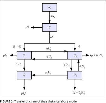
The movement of individuals into and out of each class can be described based on the model diagram. The spread of substance abuse is therefore modelled like the spread of an infectious disease. Susceptibles increase as a result of recruitment of individuals from the non-core class (NP ) at a rate proportional to the number of individuals in the non-core group so that PNp is the number of individuals recruited. We assumed that the susceptibles can become drug users through contact with active drug users in classes UL and UH. A fraction Ө of new initiates were assumed to become hard drug users and enter the class UH whilst the remainder were assumed to become light drug users. We assumed a mass action contact function so that the force of infection is given by

where b is the transmission parameter and ŋ is the relative initiation ability of hard drug users when compared to light drug users. Thus in each time unit' a susceptible individual has on average  contacts that would suffice for initiation into drug use. The assumption was that hard drug users have a lower capability of generating new drug users than light drug users by a factor ŋ such that 0 < ŋ < 1. This assumption is because hard drug users manifest ill effects of substance abuse and some may have been using drugs for a long time and may be older and socially distant from potential recruits' who are usually youths. The population of light drug users is increased by a proportion (1 - 9) of those who are recruited into drug use and also when hard users revert to light drug use at a rate The population is decreased when light drug users become hard drug users at a rate a and when they quit using drugs at a rate P2. The population of hard drug users is generated by a proportion
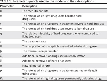
θ of susceptibles upon recruitment into drug use, when light drug users become hard drug users at a rate s and when drug users in treatment revert to hard drug use at a rate r. The population of hard drug users is decreased by removals that are related to hard drug use at a rate d1 and when hard drug users enter treatment at a rate g. The removal rate d1 models deaths and removals of individuals (e.g. as a result of imprisonment) that are drug related. Drug users in treatment are generated by hard drug users who start treatment at a rate g. This population is decreased by removals at a rate d2, when those in treatment become hard drug users at a rate r and when they permanently quit using drugs at a rate P1. The population of permanent quitters is increased when light drug users permanently quit using drugs at a rate P2, as well as when drug users in treatment quit using drugs permanently at a rate P1. We assumed that individuals in each class die naturally at a rate μ. The definition of each parameter is given in Table 1.
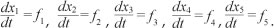
Based on the model assumptions, the model diagram and Table 1, we have the following system of differential equations:
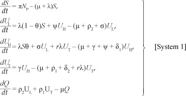
with initial conditions
S(0) ≥ 0, Ul(0) ≥ 0, Uh(0) ≥ 0, Ut(0) ≥ 0, Q(0) ≥ 0.
Basic properties
Invariant region
Because the model monitors changes in the human population, the variables and the parameters are assumed to be positive for all t ≥ 0. [System 1] will therefore be analysed in a suitable feasible region G of biological interest. The following lemma applies to the region that [System 1] is restricted to:
Lemma 1
The feasible region G defined by

with initial conditions S(0) ≥ 0, Ul(0) ≥ 0, UH(0) ≥ 0, Ut(0) ≥ 0, Q(0) ≥ 0, is positively invariant and attracting with respect to [System 1] for all t > 0.
Proof: Adding the equations of [System 1] we obtain
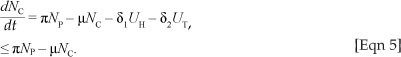
The solution NC(t) of the differential equation, [Eqn 5], has the following property 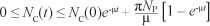 where
where
Nc(0) represents the sum of the initial values of the variables. As 
This means that  is the upper bound of NC. On the other hand, if
  then NC(t) will decrease as
  . This means that if then the solution (S(t), UL(t), UH(t), UT(t), Q(t)) enters G or approaches it asymptotically. Hence, G is positively invariant under the flow induced by [System 1]. Thus in G, [System 1] is well-posed mathematically. Hence, it is sufficient to study the dynamics of the model in G.
Positivity of solutions
For [System 1], it is important to prove that all the state variables remain non-negative so that the solutions of [System 1] with positive initial conditions will remain positive for all t > 0. We thus give Lemma 2.
Lemma 2
Given that the initial conditions of [System 1] are:
S(0) > 0, UL(0) > 0, Uh(0) > 0, Ut(0) > 0, 8(0) > 0, the solutions
S(t), Uiit), Uh(í), UT(t) and Q(t) are non-negative for all t > 0.
Proof: Assume that  and it follows from the first equation of [System 1] that
 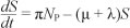 . We thus have
From the second equation of [System 1], we have
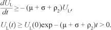
Similarly, it can be shown that
Uh(I) > 0, U(t) > 0 and Q(t) > 0 for all t > 0.
Model equilibria and stability analysis
Local stability of the drug-free equilibrium
[System 1] has a drug-free equilibrium given by:
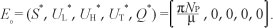
Following van den Driessche and Watmough17, the linear stability of E0 can be established using the next generation matrix method in [System 1]. Using the notations in van den Driessche and Watmough17 for our system, the matrices for the new infection terms (F) and transition terms (V) are, respectively, given by:
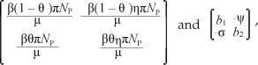
where  . It follows then that the basic reproduction number i?0 is given by the spectral
rarlinc nf /77/-1 wrlieirp T/-1 rlpnntpc fino inirprcp nf J/
We thus have
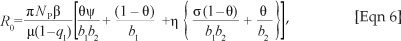
where  . R0 in this case represents the average number of secondary cases that one drug user can generate during his or her duration of drug use in a population of potential drug users. The expression of R0 is the sum of two terms representing the contribution of light drug users and hard drug users. Hence, using Theorem 2 of van den Driessche and Watmough17, we establish Theorem 1.
Theorem 1
The drug-free equilibrium point, E0 , is locally asymptotically stable if R0 < 1 , and unstable if R0 < 1 .
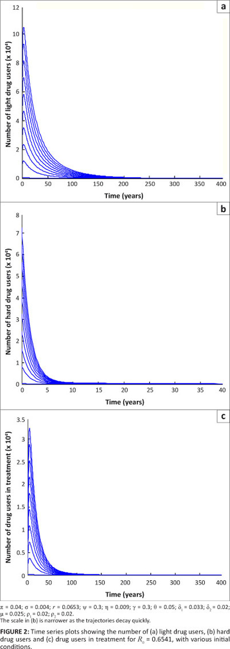
We now illustrate the above theorem numerically. We performed numerical simulations using a fourth-order Runge-Kutta scheme in Matlab.18 The aim was to verify the analytical results obtained on the stability of [System 1]. We first established the parameter values to be used in the simulations. For the purpose of these simulations, we considered hypothetical populations of one million individuals for the core group and four million individuals for the non-core group. We arbitrarily set the initial conditions for the system for illustrative purposes.
We considered the case when R0 < 1 , in particular when R0 = 0.6541. For varying initial conditions when R0 = 0.6541, the dynamics of drug users is represented by Figure 2. These results show that the population of drug users declines to zero, that is, it approaches the drug-free equilibrium. The results also show that the drug-free equilibrium is locally asymptotically stable whenever R0 < 1 . These results support Theorem 1 on the stability of a drug-free equilibrium.
Drug-persistent equilibrium
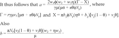
In order to determine the drug-persistent equilibrium of [System 1], we set the equations equal to zero. Let E1 = (S, UL , UH , UT , Q) represent the drug-persistent equilibrium and let

be the force of infection at steady state E1. In terms of X*, the components of E1 are
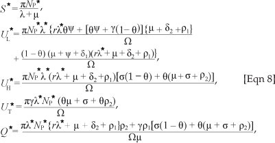

 By substituting [Eqn 8] into
[Eqn 7], and simplifying, it can be shown, after some tedious algebraic manipulations, that the non-zero equilibria of the model satisfy the following quadratic equation in terms of  *:
*:

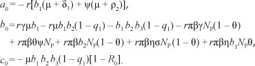
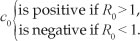
Thus, the positive drug-persistent equilibria of [System 1] are obtained by solving for l* from the quadratic equation, [Eqn 9], and substituting the results into the expressions in [Eqn 8]. Clearly, the coefficient a0 of [Eqn 9] is always negative and
We thus produce Theorem 2 on the existence of the drug-persistent equilibrium.
Theorem 2
[System 1] has four cases:
1. a unique drug-persistent equilibrium if R0 > 1
2. a unique drug-persistent equilibrium if b0 > 0 and
3. two drug-persistent equilibria if b0 > 0 and R0 < 1
4. no drug-persistent equilibrium otherwise.
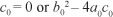
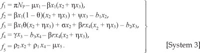
It is clear from Theorem 2 Case 1 that the model has a unique drug-persistent equilibrium whenever R0 > 1. Further, Case 3 suggests the possibility of a backward bifurcation. To check for this, we set the discriminant zero and the result solved for the critical value of R0 , giving

where R0c is a critical value of R0 , below which no drug-persistent equilibrium exists. (For an effective drug abuse control, the reproduction number should be brought below R0C. The condition R0 < 1 is not sufficient for a complete reversal of the substance abuse epidemic described by [System 1].)
Backward bifurcation
The phenomenon of backward bifurcation has been observed in many epidemiological models such as models for tuberculosis with exogenous re-infection,19,20,21 vector disease models,22 susceptible-infected-susceptible models with saturation of recoveries,23,24 and in particular, models for drug abuse.13,15 The phenomenon has epidemiological significance whereby the classical requirement of
R0 < 1 is, although necessary, no longer sufficient to end the substance abuse epidemic. Theorem 2 can be illustrated in the bifurcation diagram shown as Figure 3. Figure 3 is reminiscent of a standard backward bifurcation diagram (see for instance Dushoff25). We emphasise here that the parameter values chosen are for illustrative purposes only and may not necessarily reflect a real substance abuse phenomenon.
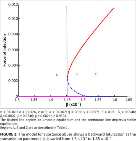
The simulation results depicted in Figure 3 show that [System 1] only has the drug-free equilibrium when R0 < R0c < 1 , two drug-persistent equilibria when R0 < R0c < 1 and one drug-persistent equilibrium when R0 > 1 , as shown by Regions A, B and C, respectively. In Region A, the drug-free equilibrium is locally asymptotically stable, whilst in Region B one of the drug-persistent equilibria is stable and the other is unstable. This result clearly shows the coexistence of two stable equilibria when R0 < R0c < 1 , confirming that [System 1] exhibits backward bifurcation. In Region C, the drug-persistent equilibrium is stable. The results shown in Figure 3 are summarised in Table 2.

The simulations were in agreement with Theorem 2. The time series plots shown in Figure 4, for different initial conditions, also reflect the existence of multiple steady states.
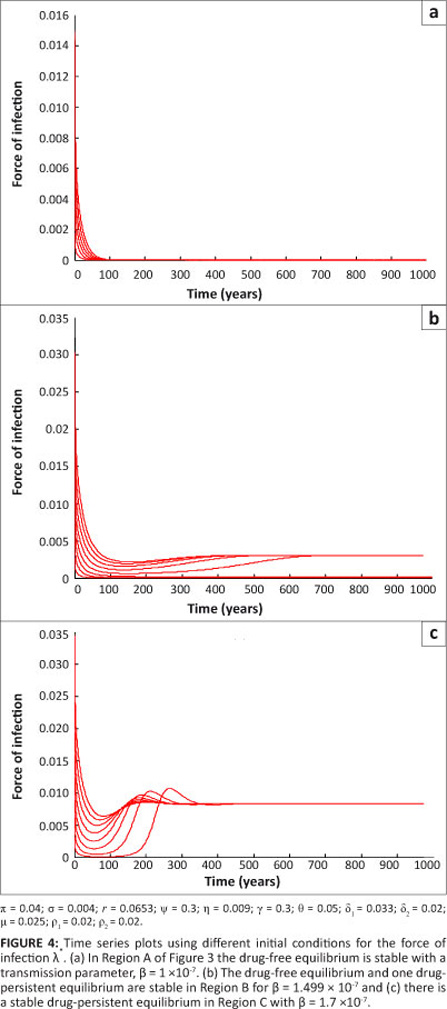
The parameter values are as given for Figure 3 with b values being within each of Regions A' B and C. It can be seen that, irrespective of the initial conditions' the force of infection stabilises to a drug-free equilibrium in Region A' one drug-persistent equilibrium and one drug-free equilibrium in Region B and to a drug-persistent equilibrium in Region C. Lemma 3 is thus established.
Lemma 3
[System 1] undergoes backward bifurcation when Case 3 of Theorem 2 holds and R0C < R0 < 1.
The role of relapse
One of the major problems relating to treatment for substance abuse is the relapse of those under treatment into hard drug use. We considered the situation in which there is no relapse to hard drug use for the sake of comparison with the case in which relapse occurs. In this situation we considered the case of r = 0, such that [System 1] reduces to
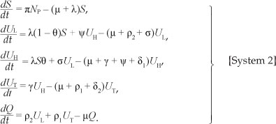
[System 2] has the same drug-free equilibrium point as [System 1]. The drug-persistent equilibrium can be obtained by considering quadratic equation, [Eqn 9], when r = 0. The coefficients a0, b0 and c0 in [Eqn 9] reduce to:
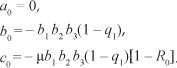
In this case, the force of infection at the steady state is X = x[R0 - 1], which is positive when R0 > 1. Then one can show that the drug-persistent equilibrium
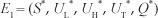
exists and is unique. S*, UL*, UH*, UT * and Q* are given by:
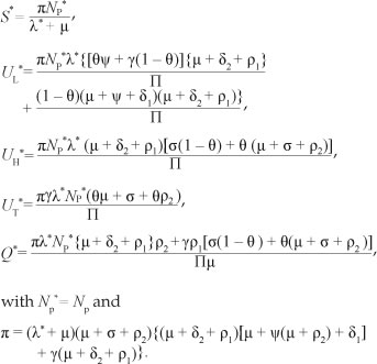
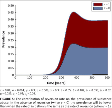
Hence, in this case (with r = 0), no drug-persistent equilibrium exists whenever R0 < 1. It follows that, owing to the absence of multiple drug-persistent equilibria for [System 1] with r = 0 and R0 < 1, a backward bifurcation is unlikely for [System 1] with r = 0 and R0 < 1. Figure 5 shows the contribution of the relapse rate r on the prevalence of drug use. In the presence of relapse, the prevalence of drug use is higher. It is important to note that when r = 0, the ability of drug users not in treatment to recruit initiates from the susceptible population is the same as the ability to recruit from individuals in treatment.
Global stability of the drug-free equilibrium
The absence of multiple drug-persistent equilibria when r = 0, suggests that the drug-free equilibrium of [System 1] is globally asymptotically stable when R0 < 1. We thus produce Theorem 3.
Theorem 3
Consider [System 2] with r = 0. The drug-free equilibrium is globally asymptotically stable in G whenever R0 < 1.
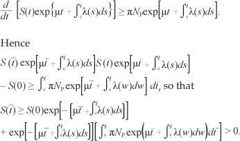
Proof: Let us consider the following Lyapunov candidate function:
where a1 and a2 are positive constants to be determined. Its time derivative along the trajectories of [System 2] satisfies
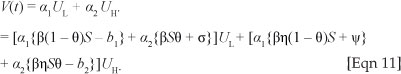
The constants a1 and a2 are chosen such that the coefficient of UH is equal to zero. Thus, one can easily show that 
Because  after substituting a1 and a2 in [Eqn 11], we obtain
  .
.
Furthermore V(t) = 0 when R0 = 1, that is, when UL = UH = UT = Q = 0. By LaSalle's invariance principle, the largest invariant set in G, contained in  is reduced to the drug-free equilibrium. This pro ves the global asymptotic stability of E0 in G (see Bhatia and Szegõ26, Theorem 3.7.11, page 346).
Local stability of the drug-persistent equilibrium
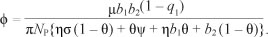
We determined the stability of the drug-persistent equilibrium and further investigated the possibility of backward bifurcation as a result of the existence of multiple equilibria as indicated in Theorem 2 Case 3. The stability analysis of the drug-persistent equilibrium point required us to determine the eigenvalues of the Jacobian matrix evaluated at the drug-persistent equilibrium. As expressing drug-persistent equilibria explicitly is complicated for [System 1], the calculation of eigenvalues is mathematically cumbersome. So we used the centre manifold theory as presented by Castillo-Chavez and Song20. To apply this method, we first changed the variables of [System 1] such that  with
with
[System 1] then becomes
We choose 4> = P as the bifurcation parameter. We thus equate R0 = 1 and obtain
The Jacobian of [System 3] at drug-free equilibrium £0 when  , is given by
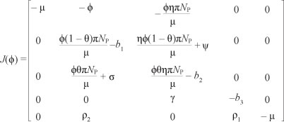
We note that the Jacobian J of the linearised system has a simple zero eigenvalue. We can thus use the centre manifold theory to analyse the dynamics of [System 3]. The right eigenvector associated with zero eigenvalue is given by w = w2, w3, w4, w5)T, where

and (.)T denotes a vector transpose. Further, J(*) has a corresponding left eigenvector v = (v1, v2, v3, v4, v5)t, where
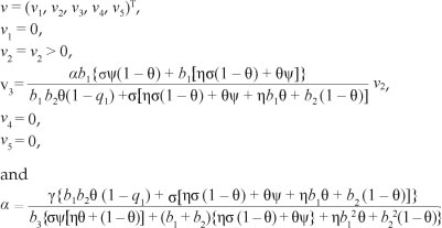
We note that all the eigenvectors are positive except for w1 and the value of a is chosen such that v. w = 1 . In order to establish the local stability of E1, we used Theorem 4 proveninCas tillo-Chavez and Song20 and adopted the use of a and b as in Castillo-Chavez and Song20. In particular, because v1 = v4 = v5 = 0,
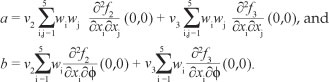
To compute the value of a and b, we first computed the nonzero second-order partial derivatives of [System 3] at drug-free equilibrium such that,
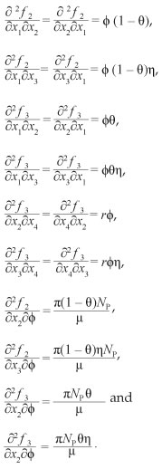
Hence the sign of a depends on the value of r and X, such that if Γ > X then a > 0 and if Γ < X then a < 0 whilst b > 0.
We thus obtain Theorem 4.
Theorem 4
If Γ > X, then [System 1] has a backward bifurcation at R0 = 1 . Alternatively, if Γ < X, then [System 1] undergoes forward bifurcation and the drug-persistent equilibrium is locally asymptotically stable for R0 > 1 but close to one.
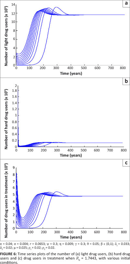
Further, using the same initial conditions when R0 = 1.7443, the population of drug users tends to a drug-persistent equilibrium in Figure 6. This pattern indicates that, irrespective of the initial conditions, the population of drug users eventually settles at the drug-persistent equilibrium with increasing time. This result is in agreement with Theorem 4.
The role of key parameters
It is also important to investigate how some key parameters jointly influence the epidemic. This investigation was performed using contour plots. In Figure 7, contours of R0 are plotted as a function of transition rates s and p2 in Figure 7a, p2 and y in Figure 7b, g and p2 in Figure 7c and g and y in Figure 7d.
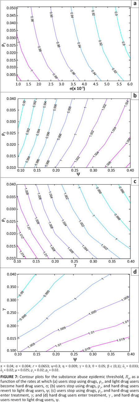
Based on the parameter values used in the simulation, Figure 7 shows that increasing s, p2 and g reduces the model reproduction number, whilst increasing y increases R0. This pattern indicates that R0 is a decreasing function of s, p2 and g, and is an increasing function of y. These results can also be obtained by performing a sensitivity analysis on R0. According to the model, to decrease the reproduction number, it is thus necessary to increase the rate at which individuals become hard drug users, the rate at which they permanently quit and the rate at which they are rehabilitated. This result makes sense as increasing forward progression rates eventually leads to more individuals quitting. The significance of increasing s to fight the epidemic is an outcome of the model formulation for two reasons. Firstly, hard drug users have been assumed to be less effective recruiters and secondly, the class of hard drug users is the entry point into treatment programmes. It is thus advantageous according to the model, for identification purposes, that an individual remains a light drug user for only a short time. In reality, this result remains debatable.
Application of the model
We applied the model to data on methamphetamine abuse in the Western Cape. [System 1] was fitted to the data for individuals who attended specialist treatment centres in the Western Cape. This data is collected every 6 months by the South Africa Community Epidemiology Network on Drug Use2 for individuals who attend specialist treatment centres in the Western Cape. The data on treatment demand trends was used to model the growth of individuals in the UT class in our model. The data for the growth of methamphetamine users in the Western Cape is given in Table 3. Table 3 includes all individuals who use methamphetamine as their primary and secondary substance of abuse.
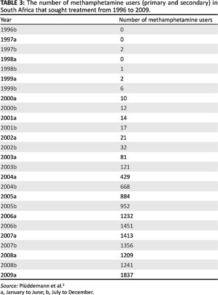
As the data is collected at 6 monthly intervals, the letter 'a' represents the first 6 months of the year (January to June) and 'b' represents the second 6 months (July to December). Because of the unavailability of data on transmission and progression rates, we estimated most of the parameters' which makes the setting of initial conditions difficult. Nevertheless, for the purpose of the simulations and illustrating the usefulness of the model' we assumed an initial population of one million for the population of individuals who are prone to become methamphetamine abusers. We set the natural death rate of 0.025.15
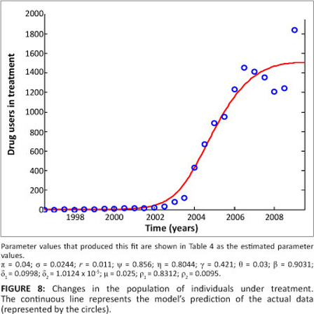
Many parameters are known to lie within limits. Only a few parameters are known exactly and it is thus important to estimate the others. The estimation process attempts to find the best accordance between the computed and observed data. The estimation can be carried out by 'trial and error' or by the use of software programs that are designed to find parameters that give the best fit. Here, the fitting process involved the use of the least squares curve fitting method. A Matlab18 code was used where unknown parameter values were given a lower and upper bound from which the set of parameter values that produced the best fit were obtained. The parameter values obtained from the fitting are shown in Table 4.
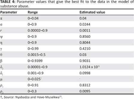
Figure 8 is a graphical representation of the model fitted to the data for individuals seeking treatment for methamphetamine abuse. As can be seen in Figure 8, the model fits well with the data.
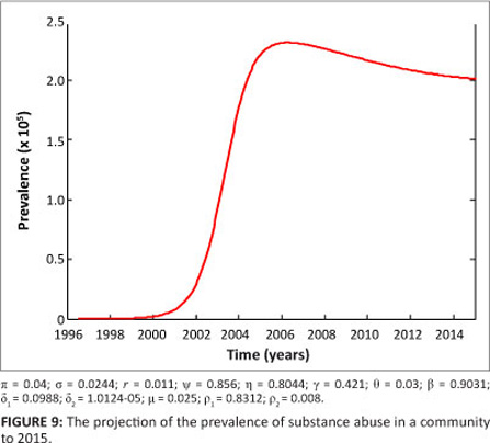
For planning and management of interventions, it is important to project the prevalence of the methamphetamine epidemic over a number of years. In our case, we chose 5 years. The projected prevalence over 5 years to 2015 is shown in Figure 9. The model projection shows that there will be a gradual decrease in prevalence. For the given parameter values, the prevalence declines from a peak value of approximately 2.3x10⁵ to 1.9x10⁵ over a period of 5 years. This estimation, of course, assumes that the dynamics remain the same over the entire period.
Discussion
We modified the compartmental deterministic model of Nyabadza and Hove-Musekwa15 to incorporate slow and fast progression of initiates and a cycle of light and hard drug use. We also included individuals who permanently stop using drugs and relapse for those under treatment. Relapse was considered synonymous to re-infection in epidemiological models. Our model was used to gain some insights into the dynamics of substance abuse. We established the local and global stability of the drug-free equilibrium. We noted that the drug-free equilibrium point is locally stable whenever R0 < 1. Also, the model has a unique drug-persistent equilibrium whenever R0 > 1, which shows persistence of substance use in the community. For some specific conditions established in Theorem 2, the model exhibits backward bifurcation and some bifurcation diagrams are presented in Figures 3 and 4.
The numerical results suggest that the spread of substance abuse can be controlled through a reduction in the relapse rate y, increasing interventions at the light drug users' phase and increasing the uptake rates into treatment. The existence of backward bifurcation in our model is indicative of complex dynamics. It is not sufficient to reduce R0 below unit to control the substance abuse epidemic but rather the value of R0 should be reduced to below R0c. It was shown that backward bifurcation is caused by relapsing to hard drug use when individuals in treatment are lured back into substance abuse by light drug users. The process remains a subject of debate as individuals in treatment are more likely to revert to drug use without due influence. The model thus suggests that strengthening of treatment programmes to prevent relapse is vital.
As with many models, the model presented in this article should be treated with circumspection because of the assumptions made and the difficulty in the estimation of the model parameters. As part of future work to improve the model in this article, the model considered here can be refined to incorporate drug users who start using drugs on their own without having contact with other drug users; the impact of behavioural changes induced by campaigns; age structure; and recruitment by drug lords. The model can also be refined for a specific substance of abuse and be fitted to data. Despite its shortcomings, the model provides useful insights into the possible impact of treatment and relapse in communities struggling with substance abuse.
Acknowledgements
A.S.K. appreciates the support of SACEMA in the production of the manuscript. F.N. acknowledges with gratitude the Department of Mathematical Sciences for its support in the production of this manuscript.
Competing interests
We declare that we have no financial or personal relationships which may have inappropriately influenced us in writing this article.
Authors' contributions
A.S.K. was the main author of the manuscript, which is part of an MSc thesis. A.S.K. designed the model, performed the analysis and wrote the manuscript. F.N. supervised the research, and helped with the simulations and revisions.
References
1. Lineberry TW, Bostwick JM. Methamphetamine abuse: A perfect storm of complications. Mayo Clin Proc. 2006;81:77-84. http://dx.doi.org/10.4065/81.1.77, PMid:16438482 [ Links ]
2. Plüddemann A, Dada S, Parry C, et al. Monitoring alcohol and substance abuse trends in South Africa. SACENDU Research brief. 2010;13(2):1-16. [ Links ]
3. Parry CDH, Dewing S, Petersen P, et al. Rapid assessment of HIV risk behavior in drug using sex workers in three cities in South Africa. AIDS Behav. 2009;13(5):849-859. http://dx.doi.org/10.1007/s10461-008-9367-3, PMid:18324470 [ Links ]
4. Wechsberg WM, Luseno WK, Karg RS, et al. Alcohol, cannibis, and methamphetamine use and other risk behaviours among Black and Coloured South African women: A small randomized trial in the Western Cape. Int J Drug Policy. 2008;19:130-139. http://dx.doi.org/10.1016/j.drugpo.2007.11.018, PMid:18207723, PMCid:2435299 [ Links ]
5. Parry CDH. Substance abuse intervention in South Africa. World Psychiatry. 2005;4:34-35. PMid:16633501, PMCid:1414718 [ Links ]
6. Rossi C. Operational models for the epidemics of problematic drug use: The Mover-Stayer approach to heterogeneity. Socio Econ Plan Sci. 2004;38:73-90. http://dx.doi.org/10.1016/S0038-0121(03)00029-6 [ Links ]
7. Rossi C. The role of dynamic modelling in drug abuse epidemiology. Bull Narc. 2002;LIV:33-44. [ Links ]
8. Mulone G, Straughan B. A note on heroin epidemics. Math Biosci. 2009;218:138-141. http://dx.doi.org/10.1016/j.mbs.2009.01.006, PMid:19563739 [ Links ]
9. De Alarcon R. The spread of a heroin abuse in a community. Bull Narc. 1969;21:17-22. [ Links ]
10. Hunt LG, Chambers CD. The heroin epidemics. New York: Spectrum Publications Inc.; 1976. [ Links ]
11. Mackintosh DR, Stewart GT. A mathematical model of a heroin epidemic: Implications for control policies. J Epidemiol Community Health. 1979;33:299-304. http://dx.doi.org/10.1136/jech.33.4.299 [ Links ]
12. Sharomi O, Gumel AB. Curtailing smoking dynamics: A mathematical modelling approach. Appl Math Comput. 2008;195:475-499. http://dx.doi.org/10.1016/j.amc.2007.05.012 [ Links ]
13. White E, Comiskey C. Heroin epidemics, treatment and ODE modelling. Math Biosci. 2007;208:312-324. http://dx.doi.org/10.1016/j.mbs.2006.10.008, PMid:17174346 [ Links ]
14. Burattini MN, Massad E, Coutinho FAB. A mathematical model of the impact of crack-cocaine use on the prevalence of HIV/AIDS among drug users. Math Comput Model. 1998;28:21-29. http://dx.doi.org/10.1016/S0895-7177(98)00095-8 [ Links ]
15. Nyabadza F, Hove-Musekwa SD. From heroin epidemics to methamphetamine epidemics: Modelling substance abuse in a South African province. Math Biosci. 2010;225:132-140. http://dx.doi.org/10.1016/j.mbs.2010.03.002, PMid:20298703 [ Links ]
16. Hadeler KP, Castillo-Chavez C. Core group model for disease transmission. Math Biosci. 1995;128:41-55. http://dx.doi.org/10.1016/0025-5564(94)00066-9 [ Links ]
17. Van den Driessche P, Watmough J. Reproduction numbers and sub-threshold endemic equilibria for compartmental models of disease transmission. Math Biosci. 2002;180:29-48. http://dx.doi.org/10.1016/S0025-5564(02)00108-6 [ Links ]
18. Matlab. Version 7.01. Natick, MA: Mathworks; 2004. [ Links ]
19. Bhunu CP, Garira W, Mukandavire Z, Magombedze G. Modelling the effects of pre-exposure and post-exposure vaccines in tuberculosis control. J Theor Biol. 2008;254:633-649. http://dx.doi.org/10.1016/j.jtbi.2008.06.023, PMid:18644386 [ Links ]
20. Castillo-Chavez C, Song B. Dynamical models of tuberculosis and their applications. Math Biosci Eng. 2004;1:361-404. [ Links ]
21. Feng Z, Castillo-Chavez C, Capurroe A. A model for tuberculosis with exogenous re-infection. Theor Popul Biol. 2000;57:235-247. http://dx.doi.org/10.1006/tpbi.2000.1451, PMid:10828216 [ Links ]
22. Garba S, Gumel A, Bakar M. Backward bifurcation in dengue transmission dynamics. Math Biosci. 2008;215:11-25. http://dx.doi.org/10.1016/j.mbs.2008.05.002, PMid:18573507 [ Links ]
23. Cui J, Mu X, Wan H. Saturation recovery leads to multiple endemic equilibria and backward bifurcation. J Theor Biol. 2008;254:275-283. http://dx.doi.org/10.1016/j.jtbi.2008.05.015, PMid:18586277 [ Links ]
24. Sharomi O, Poddler CN, Gumel AB, et al. Role of incidence function in vaccine-induced backward bifurcation in some HIV models. Math Biosci. 2007;210:436-463. http://dx.doi.org/10.1016/j.mbs.2007.05.012, PMid:17707441 [ Links ]
25. Dushoff J. Incorporating immunological ideas in epidemiological models. J Theor Biol. 1996;180:181-187. http://dx.doi.org/10.1006/jtbi.1996.0094, PMid:8759527 [ Links ]
26. Bhatia NP, Szegö GP. Stability theory of dynamical systems. Berlin: Springer-Verlag; 1970. [ Links ]
 Correspondence to:
Farai Nyabadza
Postal address:Private Bag X1, Matieland, South Africa
Email: nyabadzaf@sun.ac.za
Received: 04 Mar. 2011
Accepted: 08 Nov. 2011
Published: 16 Mar. 2012

