


Servicios Personalizados
Articulo
 Inglés (pdf)
 Articulo en XML
 Referencias del artículo
Indicadores

Links relacionados
-
 Citado por Google
 -
 Similares en Google
Compartir

 Permalink
South African Journal of Science
versión On-line ISSN 1996-7489
versión impresa ISSN 0038-2353
S. Afr. j. sci. vol.107 no.5-6 Pretoria may./jun. 2011
http://dx.doi.org/10.4102/sajs.v107i5/6.356
RESEARCH ARTICLE
A method for calculating the variance and confidence intervals for tree biomass estimates obtained from allometric equations
Alecia Nickless; Robert J. Scholes; Sally Archibald
Council for Scientific and Industrial Research, Pretoria, South Africa
ABSTRACT
The need for accurate quantification of the amount of carbon stored in the environment has never been greater. Carbon sequestration has become a vital component of the battle against global climate change, and monitoring and quantifying this process are major challenges for policymakers. Plant allometric equations allow managers and scientists to quantify the biomass contained in a tree without cutting it down, and therefore can play a pivotal role in measuring carbon sequestration in forests and savannahs. These equations have been available since the beginning of the 20th century, but their usefulness depends on the ability to estimate the error associated with the equations - something which has received scant attention in the past. This paper provides a method based on the theory of linear regression and the lognormal distribution to derive confidence limits for estimates of biomass derived from plant allometric equations. Allometric equations for several southern African savannah species are provided, as well as the parameters and equations required to calculate the confidence intervals. This method was applied to data collected from a sampling campaign carried out in a savannah landscape at the Skukuza flux site, Kruger National Park, South Africa. Here the error was 10% of the total site biomass for the woody biomass and 2% for the leaf biomass. When the data were split into individual plots and used to estimate site biomass (as would occur in most sampling schemes) the error increased to 16% and 12% of the woody and leaf biomasses, respectively, as the sampling errors were added to the errors in the allometric equation. These methods can be used in any discipline that applies allometric equations, such as health sciences and animal physiology.
Introduction
Allometric equations that relate components of aboveground tree biomass to stem dimensions are almost universally used to obtain estimates of biomass in forests, woodlands and savannahs.1 The approach has application in many areas, including resource inventories, assessing the spatial distribution of carbon,2 and comparisons in biomass allocations between different species of trees or between the same species under different circumstances.3,4 Destructive sampling of the entire aboveground mass of trees is a costly, difficult and labour-intensive process, and it results in the removal of the trees. The preferred method for estimating the biomass of individual trees or whole stands is therefore to make use of the strong relationships between the stem diameter near the ground (conventionally, but not necessarily, at breast height) and the mass of biomass components, such as wood and leaves. These relationships vary within and between species, and are time-consuming and difficult to determine. Most researchers therefore rely on published reports of species-specific allometric equations or multispecies models.5
However, if allometric relationships are to be used to calculate individual and stand biomass, it is increasingly important to have an understanding of the accuracy of these estimates by means of appropriate error calculations. This understanding is not a trivial concern5 and such error calculations have often been ignored in studies that use allometric relationships to calculate stand biomass. For example, an intensive study was carried out to determine how well biomass estimates from an allometric equation available in the literature estimated woody biomass by comparing the calculated biomass to the measured biomass of trees which were destructively sampled.6 It was shown that the equation consistently underestimated the biomass, but there were no confidence intervals associated with the estimates, and therefore it is difficult to conclude if this is a real underestimation or if the difference could be explained by the error in the estimate. The error typically has two main components: the uncertainty resulting from an incomplete sampling of the stems within a stand, and the uncertainty resulting from errors in the allometric relationships applied. The latter component of the error has been almost universally ignored, and is the focus of this paper.
The most common form for the allometric equation is y = axb, referred to as a power function, where y is the wood mass, x is the stem diameter, and a and b are the scaling parameters.5,7,8 This equation can be turned into a linear equation ('linearised') by applying the natural logarithm to both sides: ln(y) = ln(a) + bln(x). These techniques assume that ln(y) = ln(a) + bln(x) + ε*, where ε* is the random error and is assumed to be normally distributed.
In reporting plant allometry relationships, the errors in the estimation of biomass are generally not adequately quantified.5 Together with the regression coefficients, authors typically also report the sample size and the coefficient of determination (R2). Less frequently, authors provide the range in the diameters measured. We will show in this paper that these metrics do not give enough information about the errors associated with the predicted values from the regression, that is, there is not enough information to assess how well the values were predicted to allow uncertainty ranges to be calculated. When estimates of plant biomass are aggregated to stand level, the errors in the biomass estimation become aggregated as well, and the size of the error can become non-negligible. It therefore is important to obtain confidence intervals for the biomass estimates.
Zianis5 proposed using the delta method based on the second order Taylor approximation of the power function to obtain variance estimates for the predicted biomass. In this approach, the biomass, y, is treated as a straight transformation of the diameter, x, through the power function, y = axb. The coefficients are obtained from the literature and the estimate for the variance is then a function of these coefficients and the mean and variance of the diameters measured. Therefore, the error in the estimation of biomass is ignored, and the resulting variance is a function of the variance in the measured stem diameter. This variance only describes the expected variability in the biomass at the measured site if the power function between diameter and biomass can be assumed to hold exactly. As the relationship between stem diameter and biomass is generally very strong (in the order of 96% variance explained), this is a fair assumption when estimating biomass from a single stem diameter. But when biomass estimates for a stand or plot are made by aggregating the estimates from many stems, this assumption is less likely to hold, as the errors become aggregated as well. Moreover, the second order Taylor expansion only gives an approximation of the variance, and therefore introduces an additional source of error.9
Alternatives to linear regression techniques are available for obtaining allometric relationships for tree biomass. An example is the smearing estimator proposed by Duan10. The smearing estimator can be used to obtain predictions in the original scale, without the assumption of normality. Therefore this provides a non-parametric estimate of biomass from the fit of the linear regression. This estimate has been shown to be consistent under mild regulatory conditions, as well as efficient relative to parametric estimates.10 This makes the smearing estimator very appealing as an alternative to back transforming the log estimate. The difficulty in using this estimate lies in obtaining a variance or standard error for the predicted value. Ai and Norton11 proposed a technique based on the delta method for obtaining the standard error of the predicted value. This method involves a large number of additional calculations, and requires that the full data set and residuals be available from the original regression fitting. For a full derivation, refer to Ai and Norton11, who provide estimates under the assumptions of both homoscedastic and heteroscedastic variances. Because this method of obtaining confidence bands for predicted values relies on the delta method, and because of the large number of calculations required to obtain the standard error for each predicted value, as well as the large amount of information required from the original regression fitting which would be used each time a new predicted value was calculated, the smearing method is unlikely to become a popular method for obtaining biomass predictions.
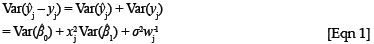
Heteroscedasticity - where the variance depends on the regressors - is a known problem for biomass allometric relationships.12 Log transforming the equation is one method of stabilising the variance.13 Alternatively, weighted regression can be substituted for the standard linear regression method. In a weighted least squares regression, yi = β0 + β1x1 + εi, where εi is assumed to be normally distributed with zero mean and variance equal to σ2wi-1.14 To obtain the regression estimators, Σwi(yi - β0 - β1x1)2 needs to be minimised. In order to implement weighted least squares regression, it is necessary for the weights to be known or the variance function to be known, which can then be used to estimate the weights from the observed data. Once the regression coefficients are estimated, obtaining a predicted value proceeds in the same fashion as for an ordinary least squares regression. To obtain a prediction interval, the variance of yj- yj, where yj is predicted from xj, is required:
Therefore, the weight of the jth predicted value is required in order to obtain a prediction interval. This requires that either the weights are known, or the weights are a known function of x and can be calculated. The danger of using weighted least squares estimates is that most of the theory developed assumes that the weights are known. Estimating the weights introduces additional uncertainty, and it is unclear how this adds to the error of the predicted values.13
The importance of accurate tree biomass estimates, and measures of this accuracy, are likely to increase in the future as schemes for payment for carbon sequestration in forests become more widespread. Allometric techniques based on relatively easily acquired field information are a realistic option for carbon accounting, but only if the associated errors can be quantified.
In this paper, we propose a method, derived from regression theory and the theory of the lognormal distribution, of assessing the error in biomass estimates obtained from allometric equations. The details and advantages of this method are described, and illustrated using allometric relationships estimated for savannah species in southern Africa.
Methodology
The general form of the simple linear regression equation is:

where i is the subject (individual stem) index, yi is the response variable, xi is the predictor variable, β0 and β1 are the regression coefficients, and εi is the error. It is assumed that the error is normally distributed with zero mean and constant variance. The constant variance assumption implies that, across the range of x values, the variability in the error does not change.
For estimating tree biomass from stem diameter, the simple linear regression equation is often modified by assuming that the logarithm of the response variable can be explained by the linear equation:

where the regression parameters superscripted by asterisks denote the log regression parameters. The assumptions previously mentioned now apply to the regression relationship with the logged variables. Therefore, ln(yi) is assumed to be normally distributed, with mean µ* = β0* + β*1 ln(xi) and variance σ2*. The fitting techniques which apply to simple linear regression can be used to obtain the regression parameters once the variables have been log transformed. This relationship is often expressed in the power form by taking exponents on both sides of the equation:

Often the error term is not shown. This is the typical form of the equation when applied to plant woody biomass.5 Another typical application of this form of the equation is the relationship between weight and height in humans.15
When choosing a method for fitting an allometric equation to the observed data, one has to take into account the fact that both the dependent variable (mass) and the independent variable (stem diameter) are measured with some error. There is much debate on whether to use the ordinary least squares (OLS), major axis or reduced major axis (RMA) methods.7,16 The OLS method is by far the most widely used and many examples of its use can be found.4,5,17,18,19,20,21 The OLS fitting method assumes that the independent variable is perfectly known, and only the dependent variable is prone to measurement error, whereas the major axis and RMA fitting methods allow both the biomass and the diameter to be measured with some error.7 McArdle16 studied the accuracy of regression estimates obtained under the three different fitting techniques and found that if the error in the independent variable was less than a third of the error in the dependent variable, then the OLS method was the most accurate. In addition, the OLS method allows for the inclusion of additional predictor variables, such as categorical variables, whereas the RMA or major axis methods are not easily employed when multiple predictors are included.22
As the relative error in stem diameter measurements is likely to be considerably smaller than the relative error in measuring woody or leaf biomass, using OLS to fit regression models for plant biomass will be justified under most circumstances. Niklas7 also states that if the R2-value is more than 0.95, then the slope estimates of the three different methods will be almost identical. Generally, R2-values for most plant biomass relationships tend to be greater than 0.90,21,23 but there are always exceptions. For these reasons, and because OLS tends to be the most widely used method, the OLS method was used for fitting regression relationships in this paper.
To test for heteroscedasticity of the residuals from the linear regressions, the studentised Breusch-Pagan test was calculated.24,25 This test specifically tests if the heteroscedasticity is such that the error variance is a multiplicative function of one or more variables, so that if x increases, the residuals fall farther and farther from the zero line. The null hypothesis for this test is that the residuals are not heteroscedastic.
If it is assumed that the natural logarithm of the response is normally distributed, then the implication is that the response itself must be lognormally distributed with mean µ = exp(µ* + σ2* /2) and variance σ2 = exp(2µ* + 2σ2*) - exp(2µ* + σ2*) .26 Note that the estimate for µ is a function of both µ* and σ2*, which is why it is not possible to simply take the exponent of the estimates of the logged response from the linear regression to obtain the estimates in the required scale, as this would result in bias.27
Statisticians and statistical software packages compute systems of linear equations (such as those that underlie linear regression analysis) using matrix algebra. A brief explanation of this convenient and efficient notation is included here for the non-specialist. The matrix of observations of the independent variable, referred to as the predictor or design matrix, is denoted X, and its transpose as X' . In the case of a simple linear regression, the first column of X is a column of ones (for the intercept), and the second column is the vector of observations of the independent variable (in the same scale as represented in the linear regression equation). A key calculation in the text that follows is (X'X)-1 which is the matrix inversion of the matrix multiplication between X and its transpose.
From regression theory it is known that the expected value (E) and variance (Var) of ln is given by:
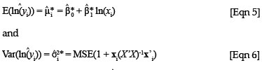
where xi = (1, ln(xi)), ln is the predicted value from a new xi value, MSE is the mean square error obtained from the original regression analysis and X is the design matrix of the original regression. In the case of a simple linear regression, the calculation of the variance of a predicted value can be simplified into easily derivable terms from the original regression data. The term X'X can be simplified to
where n is the sample size of the original regression, and the summations are applied to the predictor vector used to derive the original regression relationship, indicated by the subscript j. Therefore, if the MSE and the summary terms of X'X are available, then this closed form expression for the variance of a new predicted value can be used. A thorough explanation of linear regression theory can be found in Seber and Lee14.
The next step in the process is to obtain the predicted value of yi from µ*i = ln . This can be obtained by applying the following transformation:

Therefore, it is necessary to have an estimate of the variance for the logged prediction in order to obtain an unbiased estimate for yi. In addition, the variance of the predicted value can be obtained from the following equation26:

To obtain the 100(1 - α)% limits of a confidence interval for a predicted value, the following formulae for a lognormal variable can be used:
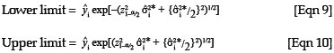
where z1-/2α is the 1 -  quantile of the standard normal distribution.28 These equations were derived based on the method described by Zou et al.28 where cofidence intervals were derived for the mean of a lognormal variable.
In general, once the biomass estimates have been obtained for individual stems, these values then get aggregated to stand level, either collectively or by species. The distribution of the sum of lognormal variables is approximately lognormal with parameters  Therefore, the estimated biomass values and their corresponding variance estimates can be summed across whole stands or across species to give the biomass estimates at a larger scale. Because the sum is still lognormally distributed, the previous formulae for confidence limits still apply, substituting
  into the place of
  and
and  into the place of
  .
.
Therefore, in order to obtain an estimate of the total aboveground biomass within a sample 'plot' (i.e. a delineated area, typically several metres squared, containing a number of stems, potentially of different species and with different diameters), the following information is required: the plot surface area, a complete list of stem diameters in the plots and the species to which each stem belongs. In addition, an allometric relationship for predicting biomass from the stem diameter is required for each species or morphological group. In order to make a rigorous estimate of the error associated with this total plot biomass, the allometric relationship must be accompanied by the following information: the sum of the squared predictor (Σ(ln xj)2), the sum of the unsquared predictor (Σln xj), the MSE and the sample size (n). If the mean and variance of the diameter values are known, then one can use a second order Taylor approximation to estimate the variance,5 but this assumes that the allometric relationships are exact. If only the sample size and R2 values are reported, it is not possible to estimate error rigorously.
Invariably, the purpose of the assessment is to estimate the biomass in a much larger area than the plot in which each stem is measured - a whole forest compartment or landscape. For this purpose, a number of replicate plots are surveyed and then extrapolated to the larger extent. This extrapolation introduces a second element of error - the spatial variability between plots. The statistical properties of sampling schemes are well understood and are described here for completeness and so that the relationship between the allometric error and spatial variability becomes clear.
It is typically assumed that the plots represent independent samples of the overall population, with a normal distribution. Under these assumptions, the mean of the sample plots is an unbiased estimator of the population value, with an error range as a result of sampling.
Stand biomass (kg/ha) = 
where Y is the sample plot biomass, np is the number of sample plots and sp is the standard deviation across the sample plots.30 (This assumes that each plot is the same size, and that the number of plots is sufficient such that the z-statistic applies rather than the t-statistic, that is, there are more than about 30 plots.)
In practice, sampling schemes may deviate from these assumptions in two important ways. Firstly, it is usually more efficient (in both statistical terms and time-and-motion terms) to estimate the biomass in a large number of small plots than a small number of large plots (although a minimum plot size should be maintained based on tree cluster size).31,32 In the extreme, this means that many of the plots will in fact have no trees, and most will have only one or two trees. Under these conditions it is unlikely that the biomass data will follow the normal distribution. If the sample plots are non-overlapping and independent, and are of the same size, then it can be assumed that the biomass per plot has a Poisson sampling distribution.33 Additional properties that justify this assumption are that the probability of observing an amount of tree biomass increases in proportion to the size of the plot, and there exists a plot size that is sufficiently small that the probability of observing tree biomass in a plot that size or smaller is virtually zero. Therefore the mean and variance of the biomass per unit area will be estimated by the sample mean of the plot biomass estimates. That means that in the previous equation, the value of sp should be approximated by  , because the variance of a Poisson variable is equal to its mean. The overall estimation error for the site biomass is the sum of the analytical error and the sampling error.30
Secondly, in some cases, the sampled area may not be an insignificant fraction of the total area, and given that the plots are typically laid out not to overlap, this is a non-replacement sample from a finite population (or is referred to as sampling without replacement), and the samples are therefore not strictly independent. As the sampled area tends towards the total area, so the sampling error tends towards zero, but the allometric error remains finite. In the extreme case where a census is taken of all the tree diameters in the area of interest, the overall estimation error will be equal to the analytical error only.
Application of method
To demonstrate this method, the stem diameters collected during a field campaign characterising the vegetation structure at the Skukuza flux site, located in the Kruger National Park, South Africa, were used to obtain the estimated biomass at the site, along with the variance estimates and 95% confidence intervals. In this example, both woody biomass and leaf biomass were estimated.
The flux tower is located at 25º01.184`S, 31º29.813`E, within a semi-arid subtropical climate. The site straddles an ecotone between a fine-leafed Acacia savannah on the somewhat more clayey downslope soils and a broad-leafed Combretum savannah on the more sandy soils of the ridge tops. A total of 24 woody species were sampled during the tree census carried out in April 2008, of which the dominant species were Combretum apiculatum, Sclerocarya birrea and Acacia nigrescens. A full site description is given elsewhere.34,35
The area in which the tree census was carried out measured 200 m x 200 m, centred on the tower itself. It was accurately demarcated into a sampling grid, where each grid cell was 50 m x 50 m. All the stems taller than 1.0 m within the entire area were measured. Species and the following stem dimensions were recorded: diameter just above the basal swelling, height, height of the lowest foliage, and maximum and minimum canopy diameters. The location of the trees was approximated (to within 1.0 m) with the assistance of the grid and a high-resolution aerial photograph.
Knowing the spatial location of each stem allowed us post hoc to sample the population at different sampling intensities, as well as to calculate the biomass for the entire surveyed area. Comparing estimates for post hoc samples to the population estimates permitted us to investigate the relative uncertainties as a result of the sampling strategy and the allometric estimates.
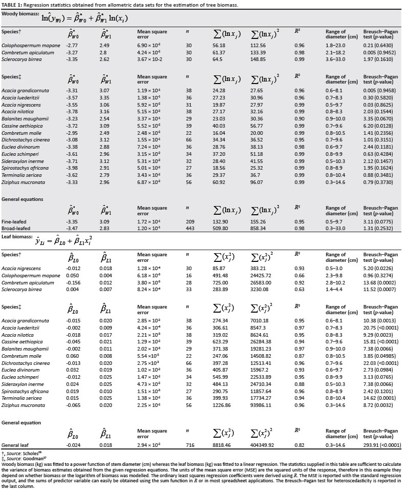
Before biomass estimates could be obtained, the available allometric data sets specific to the tree species at the site were collected and the appropriate regression parameters were calculated. To collect the allometric data sets, plant parameters (including stem diameter) were measured on the selected trees. Once these measurements were taken, the tree or branch of the tree was cut at the base. The biomass was then separated into woody and leaf biomass and then oven dried for at least 48 h. All the allometric data sets used were made available by Scholes36 and Goodman37. Both of these authors gave access to their original data, and therefore the regression coefficients and required regression statistics could be derived. Originally, only the regression coefficients, R2-values, sample size and range of stem diameters were reported.
Table 1 gives a summary of the regression results as well as the source of the original data set. The regression coefficients were derived using R open-source statistical software (http://www.r-project.org). The equation fitted to woody biomass was:

where yWi is the dried woody biomass in kilograms, xi is the stem diameter in centimetres,  and β*W 1 are the regression coefficients for the logged woody biomass and ε*Wi is the error in the estimation of logged woody biomass.
The equation fitted to leaf biomass was:

where yLi is the leaf biomass in kilograms, βL0 and βL1 are the regression coefficients for leaf biomass and εLi is the estimation error. It was found that a linear form of the relationship fits the data better than a power equation for leaf biomass, and that a relationship with the square of stem diameter fits better than the unsquared diameter, which can be explained because tree volume should scale with the cross-sectional area of the trunk. (Scholes36 and Chidumayo38 have also reported linear equations for leaf biomass.)
To obtain the variance estimates for the leaf biomass, a similar approach as described above for the logged regression equation can be implemented, but it is now not necessary to make the adjustments for the lognormal distribution. The estimate for the variance of yLi , when the relationship is in the form of a simple linear regression, is:

where xi = (1, x2 i), and X'X can now be simplified to  . The estimate for
  will be in kilograms, and therefore the variance term will be in squared kilograms.
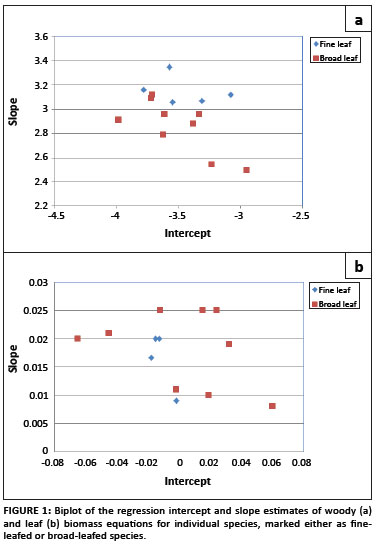
Allometric data sets were not available for all tree species present at the site, and therefore it was necessary to derive general equations from the data sets which were available for other savannah tree species. For the woody biomass general equation, a biplot of the regression parameters for the species-specific equations showed two clear groups: one applicable to broad-leafed species and the other to fine-leafed species (Figure 1), and therefore two separate general equations were derived. The species data sets used to derive the woody biomass equation for fine-leafed trees were A. nigrescens,36 A. nilotica, A. grandicornuta, A. luederitzii and Dichrostachys cinerea.37 To derive the equation for the broad-leafed species, allometric data sets for C. apiculatum, S. birrea, Colophospermum mopane,36 C. molle,Euclea schimperi, E. divinorum,Sideroxylon inerme, Spirostachys africana, Terminalia sericea, Balanites maughamii, Cassine aethiopica and Ziziphus mucronata37 were used. When the regression parameters of the leaf biomass equations were plotted against each other, no clear groups were distinguishable (Figure 1), and therefore only one general equation for leaf biomass was derived, pooling the data from all available species.
The derived regression equations, as well as the additional regression statistics, were used to obtain biomass estimates and their variances based on the stem diameter measurements taken at the Skukuza flux site.
Table 1 includes the Breusch-Pagan test for heteroscedasticity. The residuals under the woody biomass equations, where the logarithm of biomass was modelled, performed well under the Breusch-Pagan test, with only Cassine aethiopica obtaining a significant result. This species was not present at the Skukuza flux site. This indicates that logging the woody biomass sufficiently accommodates heteroscedasticity in the data. The residuals under the leaf biomass equations performed poorly in terms of heteroscedasticity, most likely because biomass was not logged in this instance. As logging the leaf biomass data leads to poorer fits of the regression line, weighted least squares regression could potentially result in better variance estimates for the predicted values without the need to log the leaf biomass, but this would require strong assumptions about the functional form of the variance, and could reduce the accuracy of the variance estimates further if incorrectly estimated. For the sake of demonstrating how the biomass estimates are aggregated under a model assuming a linear relationship for biomass, the OLS linear regressions for leaf biomass were used.
Results of application
Of the 24 savannah tree species occurring at the site, eight of these had species-specific equations. These eight species contributed 77.5% of the total aboveground woody biomass estimated at the flux site. The woody and leaf biomass were calculated for each individual stem, and then aggregated to site level and per species. Biomass is usually expressed per unit area, and therefore the biomass estimates for each sample plot were divided by the area of the plot, and the species biomass estimates for the entire site were divided by the total site area. These results are displayed in Figures 1 and 2.
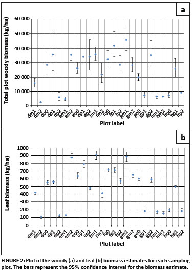
Plotting the biomass, expressed as kilograms per hectare, for the individual sampling plots, shows that there is a large amount of variability throughout the site in the distribution of the woody and leaf biomass (Figure 2). Examination of the confidence intervals for the individual plot estimates shows that, for woody biomass, the limits are not symmetrical, but rather the upper limit is more extreme than the lower limit (Figure 2). This is because the lognormal distribution is assumed to be underlying the data. In the case of the leaf biomass estimates, which are assumed to be normally distributed, the confidence intervals are symmetrical.
At this site, the plot estimates for woody biomass range between 2.5 Mg/ha and 45.5 Mg/ha. The confidence intervals range between 24% and 99% of the biomass estimate, with larger biomass estimates generally having wider intervals. The estimates for leaf biomass ranged between 0.11 Mg/ha and 0.91 Mg/ha, with confidence intervals between 6.6% and 45.8% of the biomass estimates.
There are two reasons why the larger biomass estimates would have wider confidence intervals. Firstly, if the large stand estimate is because of one or a few large individuals in the plot, the confidence interval will be wide, because as the diameter of the trees moves further outside of the range of the original regression, the confidence interval becomes wider, because the uncertainty in the estimate will be greater. In the case of a simple linear regression, the standard deviation of a predicted value can be written as39:
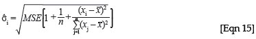
This formulation shows that the standard deviation of the predicted value from xi, σi, will get larger the farther the new x value moves from the mean of the x variables from the original regression, x. The standard deviation is the component of the confidence interval for a predicted value that determines how wide the interval will be, and therefore the confidence interval becomes wider for larger x values. In addition, in the case of the woody biomass estimates, the larger variance could be because of one or more large estimates of biomass in the plot, which would then have a large variance estimate because, under the lognormal distribution, the variance increases with increasing mean.
The second reason the confidence intervals for plots with large biomass estimates may be wide is that several stems may have been included in this plot. The error will then accumulate with each biomass prediction. If the plot contains many stems from species which require the generalised equation, or for species with poorly fitting allometric equations, then this will also result in a larger accumulated variance for the plot.
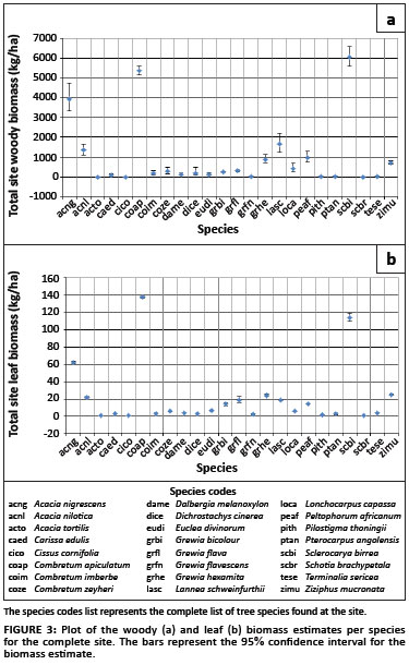
The biomass was also accumulated per species for the entire site (Figure 3). The plots show that the majority of the biomass at the site is contributed by A. nigrescens, C.apiculatum and S. birrea, obtaining woody biomass estimates (and confidence intervals) of 3.9 Mg/ha (3.3; 4.7), 5.4 Mg/ha (5.1; 5.6) and 6.1 Mg/ha (5.6; 6.6), respectively, and leaf biomass estimates of 0.062 Mg/ha (0.061; 0.063), 0.137 Mg/ha (0.136; 0.139) and 0.114 Mg/ha (0.109; 0.119), respectively.
From the census data collected of all the tree diameters at the site - a total of 6806 plant stems - the site woody biomass was calculated to be 22.93 Mg/ha (21.79; 24.13) and the leaf biomass was calculated to be 0.49 Mg/ha (0.479; 0.492). As the data collected here represent all the trees in the site of interest, there is no sampling error associated with these estimates; only the allometric error.
To demonstrate the role of the sampling error in the calculation of biomass, a sample of non-overlapping circular plots was drawn from the site. The diameter of these circular plots was 30 m. Trees falling within these plots were considered to be within the sample, and trees outside of the plots were ignored. The estimated biomass was determined for the site and for each species, along with the associated confidence limits.
To obtain the biomass estimate for the site, the biomass estimates for the sample plots were averaged to obtain the average biomass per hectare. The total error for the site biomass estimate was derived by accumulating the errors from each allometric estimation, and then adding this value to the sampling error, estimated from the square root of the average of the biomass estimates, because the data were assumed to be Poisson distributed. The same method was applied to the species biomass estimates, but in this case many of the species did not occur in each of the sampling plots, resulting in a large number of zero biomass estimates for each species.
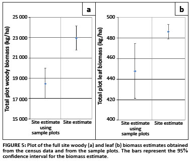
The biomass estimates obtained from the sample data compared to those derived from the census data (Figure 4), are generally quite similar, with the confidence intervals for the estimates overlapping. A notable exception is A. nigrescens, which, if the census data can be assumed to be correct, is dramatically underestimated by the sample data. L. schweinfurthii and L. capassa are also somewhat underestimated, but not quite as severely as A. nigrescens. This error could be as a result of an inappropriate sampling strategy, resulting in non-representation of A. nigrescens. The sampling strategy employed in this case placed the sampling plots on the intersection points of an evenly spaced grid, so that the points were 50 m apart. Because the trees in a savannah landscape can be clustered together, the selection of sampling plots may have been on the same scale as the natural clustering in the landscape, thereby consistently leaving out the A. nigrescens trees, which are a significant component of this system.
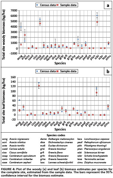
The site woody biomass estimate obtained from the sample data was 18.45 Mg/ha (16.994; 20.024), and the site leaf biomass was estimated to be 0.45 Mg/ha (0.421; 0.474) (Figure 5). Both of these estimates are slightly below the estimates obtained from the census data, but this could be explained by the non-representation of the A. nigrescens trees in the sample data.
Conclusions
The method explained in this paper provides a straightforward means of obtaining tree biomass estimates and their variances, along with confidence intervals. This method makes use of the regression theory already universally used to obtain biomass estimates, and goes further into the theory to extract the variance of predicted values. Therefore no additional assumptions are made and no additional fieldwork is required. For the widely used power law formulation of the relationship between stem diameter and woody mass, lognormal distribution theory is used to obtain appropriate estimates and asymmetric confidence intervals for the biomass estimates. Once the variance estimates are obtained for the biomass estimated from individual stems, these estimates can be accumulated by plot or by species and integrated with the uncertainties resulting from partial sampling of the spatially heterogeneous forest stand.
If this method is to be widely implemented, then future publications of tree biomass allometric relationships must report, in addition to the regression coefficients, the sum of the squared and unsquared predictor variable, the MSE and the sample size. These statistics are readily available from current statistical analysis software. Together, these parameters fully define the relationship. Where methods other than OLS are used to obtain allometric relationships, additional parameters should be reported to allow users of these equations to calculate error estimates for the biomass predictions. In the case of weighted least squares methods, parameters should be included to allow the user to calculate the weight allocated to the predictor variable (e.g. stem diameter) from which the biomass estimate is derived, so that prediction intervals can be calculated as well.
The application of this method demonstrates that errors in the estimation of biomass can result not only from the uncertainty in the relationship between stem diameter and biomass, but also from the sampling error. A poorly designed sampling scheme which results in the under-representation or over-representation of certain species can result in larger errors in the estimates than those as a result of the use of generalised allometric equations.
Allometry is not restricted to plant biomass estimation. Other examples where allometric equations (also in the form of the power function) are used for estimation include: prediction of the clearance rate (the rate at which a unit volume of water is completely cleared of particles) of a bivalve from its weight or length40; prediction of an organism's metabolic rate from its body size and temperature41; and prediction of aspects of animal behaviour, such as foraging and home range size, from body size measurements.42 This methodology can be extended to any application where a linear regression equation obtained from historic data is used to predict new data, including those applications where a logged dependent variable is used.
Acknowledgements
P. Goodman and R.J. Scholes are acknowledged for making their allometric data sets available for this publication. The Council for Scientific and Industrial Research (Pretoria, South Africa) is acknowledged for providing funding for this research.
References
1. Brown S. Measuring carbon in forests: Current status and future challenges. Environ Pollut. 2002;116:363-372. doi:10.1016/S0269-7491(01)00212-3 [ Links ]
2. Houghton RA, Lawrence KT, Hackler JL, Brown S. The spatial distribution of forest biomass in the Brazilian Amazon: A comparison of estimates. Glob Chang Biol. 2001;7:731-746. doi:10.1046/j.1365-2486.2001.00426.x [ Links ]
3. Ong JE, Gong WK, Wong CH. Allometry and partitioning of the mangrove, Rhizophora apiculata. For Ecol Manage. 2004;188:395-408. [ Links ]
4. Peichl M, Arain MA. Allometry and partitioning of above- and below ground tree biomass in an age-sequence of white pine forests. For Ecol Manage. 2007;253:68-80. [ Links ]
5. Zianis D. Predicting mean aboveground forest biomass and its associated variance. For Ecol Manage. 2008;256:1400-1407. [ Links ]
6. Cairns MA, Olmsted I, Grandos J, Argaez J. Composition and aboveground tree biomass of a dry semi-evergreen forest on Mexico's Yucatan Peninsula. For Ecol Manage. 2003;186:125-132. [ Links ]
7. Niklas KJ. Plant allometry: Is there a grand unifying theory? Biol Rev. 2004;79:871-889. doi:10.1017/S1464793104006499, PMid:15682874 [ Links ]
8. Zianis D, Mencuccini M. On simplifying allometric analyses of forest biomass. For Ecol Manage. 2004;187:311-332. [ Links ]
9. Duursma RA, Robinson AP. Bias in the mean tree model as a consequence of Jensen's inequality. For Ecol Manage. 2003;186:373-380. [ Links ]
10. Duan N. A nonparametric retransformation method. J Am Statistical Assoc. 1983;78:605-610. doi:10.2307/2288126 [ Links ]
11. Ai C, Norton, E. Standard errors for the retransformation problem with heteroscedasticity. J Health Econ. 2000;19:697-718. [ Links ]
12. Parresol BR. Modeling multiplicative error variance: An example predicting tree diameter from stump dimensions in Baldcypress. For Sci. 1993;39:670-679. [ Links ]
13. Carroll RJ, Ruppert D. Transformation and weighting in regression. New York: Chapman and Hall; 1988. [ Links ]
14. Seber GAF, Lee AJ. Linear regression analysis. Hoboken: Wiley; 2003. [ Links ]
15. García-Berthou E. On the misuse of residuals in ecology: Testing regression residuals vs. the analysis of covariance. J Anim Ecol. 2001;10:708-711. doi:10.1046/j.1365-2656.2001.00524.x [ Links ]
16. McArdle BH. The structural relationship: Regression in biology. Can J Zool. 1988;66:2329-2339. doi:10.1139/z88-348 [ Links ]
17. Chave J, Andalo C, Brown S, et al. Tree allometry and improved estimation of carbon stocks and balance in tropical forests. Oecologia. 2005;145:87-99. doi:10.1007/s00442-005-0100-x, PMid:15971085 [ Links ]
18. Henry HAL, Thomas SC. Interactive effects of lateral shade and wind on stem allometry, biomass allocation, and mechanical stability in Abutilon theophrasti (Malvaceae). Am J Bot. 2002;89:1609-1615. doi:10.3732/ ajb.89.10.1609 [ Links ]
19. Northup BK, Zitzer SF, Archer S, McMurtry CR, Boutton TW. Above-ground biomass and carbon and nitrogen content of woody species in a subtropical thornscrub parkland. J Arid Environ. 2005;62:23-43. doi:10.1016/j.jaridenv.2004.09.019 [ Links ]
20. Son Y, Hwang JW, Kim ZS, Lee WK, Kim JS. Allometry and biomass of Korean pine (Pinus koraiensis) in central Korea. Bioresour Technol. 2001;78:251-255. doi:10.1016/S0960-8524(01)00012-8 [ Links ]
21. Williams CJ, LePage BA, Vann DR, et al. Structure, allometry, and biomass of plantation Metasequoia glyptostroboides in Japan. For Ecol Manage. 2003;180:287-301. [ Links ]
22. Wainwright PC, Reilly SM. Ecological morphology: Integrative organismal biology. Chicago: University of Chicago Press; 1994. [ Links ]
23. Laclau J, Bouillet J, Gonçalves JLM, et al. Mixed-species plantations of Acacia mangium and Eucalyptus grandis in Brazil - 1: Growth dynamics and aboveground net primary production. For Ecol Manage. 2008;255:3905-3917. [ Links ]
24. Breusch TS, Pagan AR. A simple test for heteroscedasticity and random coefficient variation. Econometrica. 1979;47:1287-1294. doi:10.2307/1911963 [ Links ]
25. Koenker R. A note on studentizing a test for heteroscedasticity. J Econometrics. 1981;17:107-112. doi:10.1016/0304-4076(81)90062-2 [ Links ]
26. Crow EL, Shimizu K. Lognormal distributions: Theory and applications. New York: Dekker; 1988. [ Links ]
27. Stow CA, Reckhow KH, Qian SS. A Bayesian approach to retransformation bias in transformed regression. Ecology. 2006;87:1472-1477. doi:10.1890/0012-9658(2006)87[1472:ABATRB]2.0.CO;2 [ Links ]
28. Zou GY, Huo CY, Taleban J. Simple confidence intervals for lognormal means and their differences with environmental applications. Environmetrics. 2009;20:172-180. doi:10.1002/env.919 [ Links ]
29. Fenton LF. The sum of log-normal probability distributions in scatter transmission systems. IRE Trans Comm Syst. 1960;8:57-67. doi:10.1109/ TCOM.1960.1097606 [ Links ]
30. Pitard FF. Pierre Gy's sampling theory and sampling practice: Heterogeneity, sampling correctness, and statistical process control. 2nd ed. Boca Raton: CRC Press; 1993. [ Links ]
31. Eckblad JW. How many samples should be taken? Bioscience. 1991;41:346-348. doi:10.2307/1311590 [ Links ]
32. Kenkel NC, Podani J. Plot size and estimation efficiency in plant community studies. J Veg Sci. 1991;4:539-544. doi:10.2307/3236036 [ Links ]
33. Ripley BD. Spatial statistics. Hoboken: Wiley; 2004. [ Links ]
34. Scholes RJ, Gureja N, Giannecchinni M, et al. The environment and vegetation of the flux measurement site near Skukuza, Kruger National Park. Koedoe. 2001;44:73-83. [ Links ]
35. Archibald SA, Kirton, A, Van der Merwe MR, Scholes RJ, Williams CA, Hanan N. Drivers of inter-annual variability in Net Ecosystem Exchange in a semi-arid savanna ecosystem, South Africa. Biogeosciences. 2009;6:231-266. doi:10.5194/bg-6-251-2009 [ Links ]
36. Scholes RJ. Response of three semi-arid savannas on contrasting soils to the removal of the woody component. PhD thesis, Johannesburg, University of the Witwatersrand, 1988. [ Links ]
37. Goodman PS. Soil, vegetation and large herbivore relations in Mkuzi Game Reserve, Natal. PhD thesis, Johannesburg, University of the Witwatersrand, 1990. [ Links ]
38. Chidumayo EN. Above-ground woody biomass structure and productivity in a Zambezian woodland. For Ecol Manage. 1990;36:33-46. [ Links ]
39. Chatterjee S, Hadi AS. Regression analysis by example. New York: Wiley; 2006. doi:10.1002/0470055464 [ Links ]
40. Filgueira R, Labarta U, Fernández-Reiriz MJ. Effect of condition index on allometric relationships of clearance rate in Mytilus galloprovincialis Lamarck, 1819. Rev Biol Mar Ocean. 2008;43:391-398. [ Links ]
41. Gillooly JF, Brown JH, West GB, Savage VM, Charnov EL. Effects of size and temperature on metabolic rate. Science. 2001;293:2248-2251. doi:10.1126/science.1061967, PMid:11567137 [ Links ]
42. Dial KP, Greene E, Irschick DJ. Allometry of behaviour. Trends Ecol Evol. 2008;23:394-401. doi:10.1016/j.tree.2008.03.005 [ Links ]
 Correspondence to:
Alecia Nickless
Postal address: PO Box 395
Pretoria 0001, South Africa
Email: ANickless@csir.co.za
Received: 15 July 2010
Accepted: 07 Feb. 2011
Published: 23 May 2011
© 2011. The Authors. Licensee: OpenJournals Publishing. This work is licensed under the Creative Commons Attribution License.

