


Services on Demand
Article
 English (pdf)
 Article in xml format
 Article references
Indicators

Related links
-
 Cited by Google
 -
 Similars in Google
Share

 Permalink
South African Journal of Science
On-line version ISSN 1996-7489
Print version ISSN 0038-2353
S. Afr. j. sci. vol.105 n.11-12 Pretoria Nov./Dec. 2009
RESEARCH ARTICLES
System description of the mobile LIDAR of the CSIR, South Africa
A. SharmaI; V. SivakumarI, II, *; C. BolligI; C. van der WesthuizenI; D. MoemaI
ICSIR National Laser Centre, P.O. Box 395, Pretoria 0001, South Africa
IIDepartment of Geography, Geoinformatics and Meteorology, University of Pretoria, Pretoria 0002, South Africa
ABSTRACT
South Africa's first mobile LIDAR (LIght Detection And Ranging) system is being developed at the National Laser Centre (NLC) of the Council for Scientific and Industrial Research (CSIR) in Pretoria (25°45'S; 28°17'E). The system is designed primarily for remote sensing of the atmosphere. At present, the system is being optimised for measuring vertical atmospheric backscatter profiles of aerosols and clouds. In this paper, we describe the complete LIDAR system, including laser transmission, telescope configuration, data acquisition, data archival and post-processing.
Key words: LIDAR, atmosphere, backscatter, laser, remote sensing
Introduction
The laser radar, more popularly known as LIDAR, is becoming one of the most powerful techniques for active remote sensing of the earth's atmosphere.1 Lasers offer great advantages over other light sources in terms of peak power, as well as narrow spectral width and narrow beam width. LIDARs also offer advantages over radar, since the wavelengths used are much shorter. This enables the detection and measurement of much smaller particles (sub-micrometer diameters), such as aerosols and water vapour. Furthermore, the narrow coherent laser beam results in higher resolutions being attained.
Laser systems were deployed for atmospheric studies immediately after the demonstration of the first laser in 1960. Fiocco and Smullin2 were the first to use the laser for atmospheric studies. In 1963, using a 0.5 J Ruby laser, they obtained Rayleigh-scattered signals from the atmosphere at altitudes up to 50 km and further detected dust layers in the atmosphere. In 1963, Ligda3 made the first LIDAR measurements of cloud heights in the troposphere height region and, in 1967, Leonard4 detected Raman scattering of O2 and N2 using a nitrogen laser. A year later, Cooney5 made range-resolved nitrogen measurements up to an altitude of 3 km with a Ruby laser, and, in 1970, Inaba and Kobayasi6–8 performed laser spectral analysis of nitrogen, oxygen and several pollutants.
The DIfferential Absorption LIDAR (DIAL) technique is one which can provide the best accuracy for measuring atmospheric pollutants. The first experimental and theoretical analysis of the DIAL method was made by Schotland9,10 in 1966 and 1974. He performed the first measurements of humidity vertical profiles utilising a Ruby laser tuned to the water vapour absorption line. The first measurement of atmospheric pollutants was made by Rothe et al.,11 who detected NO2 up to distances of 4 km. By now there are several reports available on measurements of SO2 and NO2 using DIAL techniques.12–16 More recent studies have focused on simplifying the system. In 1997, Toriumi et al.17 developed a DIAL system based on solid-state lasers for NOx detection. Similarly, Fischer and Feak18 designed a compact DIAL system for atmospheric ozone measurements. In 2001, Fujii et al.19 described the advantage of using a dual DIAL system for atmospheric SO2 measurements. Since these pioneering attempts, laser remote sensing of the atmosphere has come a long way. With the development of different laser sources, improvements in detector technology and improved data collection and analysis techniques, LIDAR has become a reliable and effective tool for atmosphere research.1
In a recent internet survey,20 it was confirmed that, although LIDAR studies of the atmosphere are highly prevalent in other parts of the world, LIDAR is yet to become a state of the art system for Africa, including South Africa. Using advanced techniques and instrumentation, a mobile LIDAR system was designed and is being developed at the Council for Scientific and Industrial Research (CSIR) National Laser Centre (NLC) in Pretoria (25°45'S; 28°17'E). This paper focuses on the technical specifications of the mobile LIDAR system.
LIDAR system overview
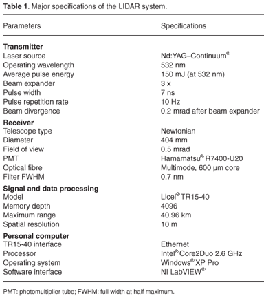
LIDAR systems can be generally divided into three main sections: a laser transmitter, an optical receiver and a data acquisition system. The complete LIDAR system is custom fitted into a van using a shock-absorber frame. The major specifications of the LIDAR system are listed in Table 1.
The transmitter and receiver are co-located, resulting in a monostatic configuration that maximises the overlap of the outgoing beam with the receiver field of view. The LIDAR system has been mounted in a van with a special shock-absorber frame. Figure 1 is a photograph of the mobile LIDAR van and a three-dimensional model of the inside of the setup. The model shows the air-filled bellows which are mounted to the van floor to provide vibration damping to the aluminium structure which supports the sensitive optical and mechanical components. Height-adjustable, hydraulic stabiliser feet have been added to the vehicle suspension to ensure stability during the measurements. When stationary, the four stabiliser feet can be extended downward, allowing the van to be completely supported and eliminating movements due to the tyres or suspension.
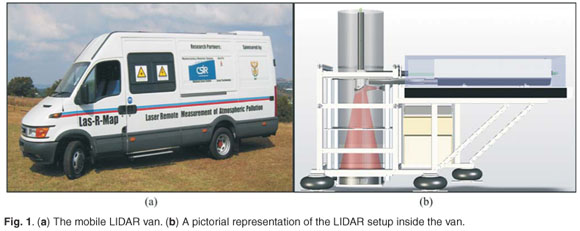
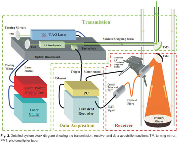
Figure 2 presents the system block diagram showing all the components. The three main sections, namely the transmission, receiver and data acquisition sections, are distinguished. The transmission section shows the laser system with turning mirrors and beam expander. The receiver section shows the receiver telescope with the primary mirror as well as the motorised translation stage and photo-multiplier tube (PMT). The data acquisition section shows the personal computer as well as the transient recorder.
Laser transmission section
The transmitter employs a Q-switched, flashlamp-pumped Nd:YAG solid-state pulsed laser (Continuum®, PL8010). Nd:YAG lasers operate at a fundamental wavelength of 1064 nm. Second and third harmonic conversions are sometimes required, depending on the application, and are accomplished by means of suitable non-linear crystals, such as potassium (K) dihydrogen phosphate (KDP). The efficiency of this conversion depends upon the quality of the crystal, and the irradiance and coherence properties of the crystal. At present, only the second harmonic (532 nm) is utilised and the corresponding laser beam diameter is approximately 8 mm.
The laser uses a Q-switch to obtain high-peak-power, short-duration laser pulses by controlling the loop gain of the optical cavity of the laser. A Q-switch is essentially a fast shutter which is located in the laser resonator. The Q-switch delay was optimised for maximum output power.
The visible, green laser beam (532 nm) is passed through a beam expander (for three-fold expansion), before being sent into the atmosphere. Due to the expansion, the transmit beam divergence is reduced from approximately 0.6 mrad to 0.2 mrad. The resultant expanded beam has a diameter of 24 mm and is then reflected upward using a flat, 45 degree turning mirror. The mirror has a diameter of 75 mm and a thickness of 8 mm. The mirror coating is specified for 532 nm and has a more than adequate damage threshold of1GWcm–2. The entire transmission setup is mounted on an optical breadboard. The optical breadboard was chosen for its enhanced damping and stiffness, which allows it to resist bending and to absorb low level vibrations. The breadboard and the entire beam path are shielded with a cover and tubing to ensure eye safety to the users and operators, as well as to reduce random scattering.
The power supply unit controls and monitors the operation of the laser. It allows the user to setup important parameters, such as the flash lamp voltage, Q-switch delay and the laser repetition rate. It also monitors system diagnostics such as the flow and temperature interlocks. General user operation and control is also available via a remote control interface. The power supply also incorporates a water to water heat exchanger which regulates the temperature and quality of water used to cool the flash lamps and laser rods. An external water cooler (MTA, M10 R407C air-cooled chiller) is employed to remove heat from the heat exchanger. The laser and cooling system is interlocked to the control unit. The laser will therefore not turn on if the cooling system is not functional or is malfunctioning. The system shutdowns if the temperature of the cooling water decreases or increases from the optimal range. The laser controller also allows for the adjustment of the pulse repetition rate from 1 Hz to 10 Hz. At present, the laser is utilised at 10 Hz.
Receiver section
The receiver system employs a Newtonian telescope configuration with a 404 mm primary mirror. The backscattered signal is first collected and focused by the primary mirror of the telescope. The signal is then focused toward a secondary 45-degree plane mirror and coupled into an optical fibre.
The primary reflecting mirror has a 2.4 m radius of curvature and a diameter of 404 mm. The mirror is coated with an enhanced aluminium substrate. The focal length of the telescope is 1.2 m. We also employed a motorised three-dimensional translation stage in order to accurately align the fibre using computer control. The beam transition and reception optics are well shielded, which further reduces background noise (Fig. 1b). The laser beam is transmitted through an inner tube (with a diameter of 50 mm), and an outer tube (with a diameter of 450 mm) that is used to shield the reception. This shield is extended to the top of the exit of the van in order to shield the receiver from random scattering.
Optical fibre
A multimode, premium-grade optical fibre is used to couple the received backscatter optical signal from the telescope to the PMT. One end of the fibre is connected to an optical baffle which receives the return signal from the telescope. The other end is connected to an optical tube with collimation optics and the PMT.
The fibre has a numerical aperture of 0.22, providing an acceptance angle of 25.4 degrees. The acceptance angle is sufficient and comparable with the solid angle provided by the curvature of the primary mirror used in the telescope. The fibre core is composed of pure silica with a high OH content, which is optimised for the UV/VIS/NIR spectrum (300 nm–1100 nm). The fibre is protected by a stainless steel jacket which provides flexibility and mechanical protection. The fibre diameter also acts as an iris and, with the use of different fibre diameters, one is able to vary the telescope's field of view.
The fibre coupling of the telescope to the detector has the advantage that it can be used for optical alignment of the fibre tip to the telescope. This is accomplished by focusing an alignment laser into the 'PMT end' of the fibre and monitoring the beam exiting the telescope. The sharpness of the focused image obtained at an extended distance away can be observed to identify the optimal position of the fibre.
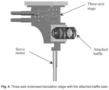
Three-dimensional translation stage and optical baffle
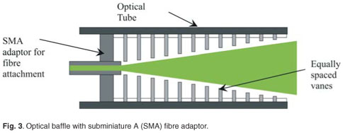
As mentioned above, one end of the fibre is located to collect the backscattered signal from the secondary mirror of the telescope. A motorised three-dimensional translation stage is used for accurate alignment of the fibre tip. The optical fibre is connected to an optical baffle (Fig. 3) which is positioned by the stage. The baffle is a mechanical system, basically consisting of an optical tube and vanes along the inner wall of the tube. Its function is to shield stray light from outside the field of view of the fibre, from the actual backscattered signal. Therefore, any light which originates outside the field of view of the fibre is allowed to make multiple reflections along the surfaces of the vanes, reducing the intensity and minimising the effect of any stray light on the signal reaching the detector.
The motorised three-dimensional stage is shown in Fig. 4. The X, Y and Z axes allow for three-dimensional alignment of the fibre tip, with respect to the field of view of the telescope, to receive the maximum backscattered signal. Each axis is controlled by DC servo motors, each having a maximum displacement of 12.7 mm (0.5 inches). The motor drivers communicate with a personal computer via USB connections using the supplied software drivers. The software interface provides all the necessary functionality, such as homing, movement to a specific desired position and a jogging function which provides incremental movement in the specified direction.
The PMT optical tube
A PMT is used to convert the optical backscatter signal to an electronic signal. The PMT is installed in an optical tube and is preceded by a collimation lens and narrow band pass filter. The tube is thermally stabilised with the use of thermoelectric cooling. This setup, including the metal box used to enclose the PMT and cooled optical tube, is shown in Fig. 5. The PMT end of the fibre enters the box and is coupled to the optical tube via a subminiature A adaptor. The backscattered signal is then collimated using a visible Achromat lens which provides minimal spherical aberration. The lens has a focal length of 10 mm and is coated for the 400 nm to 700 nm wavelength region. Using these specifications, it was calculated that a single lens would be sufficient to collimate the optical signal exiting the fibre (with a numerical aperture of 0.22) into a beam width of 6 mm diameter, which is the requirement for the 8 mm PMT.
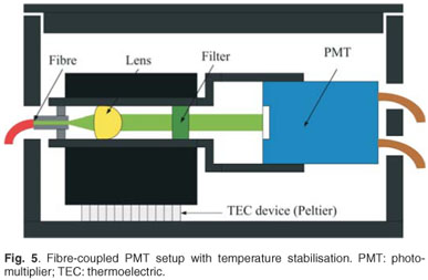
The collimated beam is then passed through a narrow band filter. The filter is a custom bandpass optical filter with a centre wavelength of 532.2 nm. The full width at half maximum (FWHM) transmission window is 0.7 nm with a maximum transmission of 64%. The filter transmission is sensitive to temperature fluctuations and therefore thermal stabilisation was incorporated into the design with the use of a Peltier element. The filter is maintained at a temperature of approximately 23°C for maximum transmission at 532 nm.
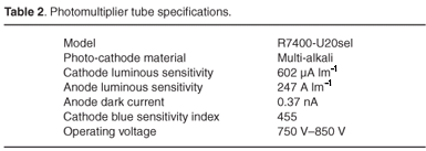
The filtered signal then enters the PMT, which is encased in a 1-inch diameter metal package to couple into the optical tube. The photomultiplier tube used is a Hamamatsu R7400-U20. It is a subminiature PMT which operates in the UV to NIR wavelength range (300–900 nm) and has a fast rise time of 0.78 ns. It is specially selected for minimal noise with an anode dark current of 0.37 nA. Typical anode dark currents for these devices range from 2–20 nA. The recommended operating voltage is 750–850 V. The PMT specifications are summarised in Table 2.
Data acquisition and archival
Data acquisition is performed by a Licel® transient recorder (TR).21 The recorder is optimised for fast repetitive photomultiplier LIDAR signals in the analog voltage range of 0–500 mV and communicates with a host computer for the storage and offline processing of data. This system is favoured due to its capability of simultaneous analog and photon counting detection, which makes it highly suited to LIDAR applications by providing a higher dynamic range.
The TR15-40 is the model that was procured. It is capable of 15 MHz sampling and has a memory depth of 4096 bins. A schematic diagram of the layout of the digitiser is shown in Fig. 6. The digitiser comprises two simultaneous detection channels, each with its own pre-amplifiers. The analog channel's amplifier is optimised for high linearity, while the photon count channel's amplifier is optimised for maximum speed and gain. An antialiasing filter selects the lower frequency range of the received signal below 7.5 MHz before it is digitised by a 12-bit A/D converter with a fast memory of 4 KB. The data is buffered in a first-in-first-out (FIFO) buffer, before being accumulated in the respective random access memory (RAM) bank.
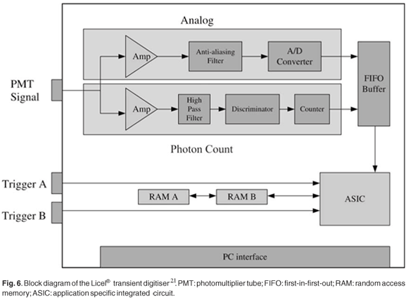
The photon count channel uses a high pass filter to select the high frequency component (>10 MHz) of the amplified PMT signal. The filtered component is then passed through a fast discriminator (250 MHz) and counter, enabling the detection of single photons.
The discriminator threshold is software adjustable from 0–100 mV. The counts are buffered in the FIFO buffer, before being recorded to RAM. The application specific integrated circuit allows for fast summation of the signals from the FIFO buffer. The recorder incorporates two triggers and two RAM banks. Depending on which trigger input is used, the buffered signal is added to the respective RAM bank. This allows for the acquisition of two repetitive channels if the signals can be measured sequentially. In DIAL applications, for example, this would be advantageous, since the backscatter of both the 'ON' and 'OFF' wavelengths can be acquired sequentially. The important specifications are tabulated in Table 3.

The Licel® system was shipped with a LabVIEW software interface that allows the user to acquire signals without the need for immediate programming. This software development environment is advantageous since it is also compatible with the three-dimensional translation stage control software. Communication with the personal computer is accomplished via Ethernet. This interface is convenient since it provides sufficient data transfer rates and eliminates the need for extra interfacing hardware.
The acquired measurements are stored in an ASCII-binary data file. The first three lines of data provide a header which describes the measurement situation and includes information such as the location, start/stop times, number of laser shots, laser repetition rate and the number of included datasets. The header is followed by the dataset description, which includes information such as whether it is a analog or photon count dataset, the PMT voltage, the laser wavelength and polarisation and the analog voltage range and photon count discriminator level. The dataset description is followed by the raw data, which is stored as 32-bit integer values separated by the ASCII equivalent of CRLF. These markers are used to determine data file integrity.
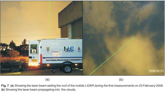
As mentioned, the Licel® data acquisition system incorporates electronics which are capable of simultaneous acquisitions of analog data and photon count data with a range resolution of 10 m. The combination of analog data and photon count data electronics greatly extends the dynamic range of the detection channel allowing the reduction or removal of neutral density filters, which in turn greatly improves the signal-to-noise ratio. An illustrative example is shown in Fig. 7, for 23 February 2008. The measurements were done at night to minimise background stellar noise. The laser was directed vertically upward into the sky as shown. The corresponding night presented a cloudy sky and there was a passage of cumulous clouds, which normally are found at lower altitudes from 3 km to 5 km, passing overhead. Since these clouds are generally optically dense, light is prevented from passing through.
The observations were carried out for approximately one and a half hours and the presence of clouds is clearly seen in the height-time-backscattered signal returns for both the analog data and photon count data, presented in Figs 8 and 9, respectively. The figures were obtained after modifying the provided Licel® – LABVIEW software. The supplied software was modified in-house to display an automatically updated height-time-backscatter colour map in real time. The advantage of such a program is that it allows the user to infer the data simultaneously while the LIDAR system is in operation. The display can be easily visualised and the available settings enable either the analog data or photon count data to be displayed, as required. The figures presented here are the raw data multiplied by the square of the altitude, commonly referred to as range-corrected signal.
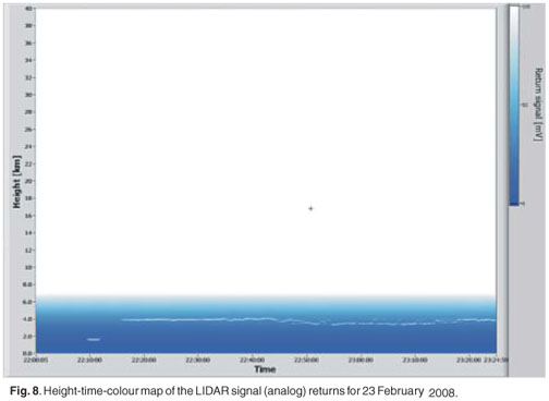
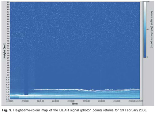
The figures clearly distinguish the cloud observation from normal scattering from background particulate matter. Sharp enhancements are observed at about 4.5 km, indicating the presence of cloud. This figure also demonstrates the capability of LIDAR to observe the cloud thickness in addition to the cloud height. This is one of the important advantages of LIDAR, in comparison with other remote-sensing measurement techniques. The advantage of having high-resolution data (10 m) further addresses the accurate detection of cloud height and thickness, which is important for studying the cloud morphology. The noisy region above 12 km is evident from the figure, but it is important to note here that the experiment was done using two neutral density filters, which prevents 99% of signal being detected. Therefore, the backscattered signal represented in these colour maps and in the height profiles corresponds to only 1% of the backscattered signal. The neutral density filters are employed to avoid PMT saturation and to investigate the maximum return signal strength. In future experiments, we will investigate removing the neutral density filters and also the use of a smaller diameter fibre (200 µm). It is expected that this will greatly improve our signal-to-noise ratio and further extend the observable altitude range of the LIDAR.
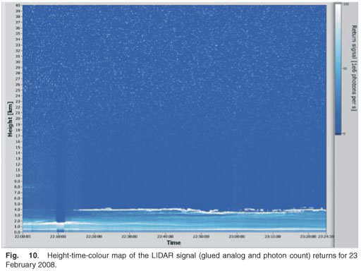
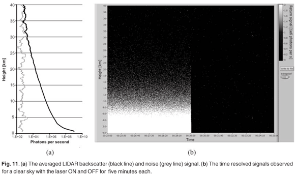
To make use of the simultaneous analog data and photon count data acquisition, post-processing is required to merge or 'glue' the datasets into a single return signal. The combined analog data and photon count signals allow us to use the analog data in the strong signal regions and the photon count data in the weak signal regions. Since the output from the analog data converter is voltage (V) and the output from the photon counter is counts or count rates (MHz) a conversion factor between those outputs needs to be determined in order to convert the analog data to 'virtual' count rate units. First the photon count data is corrected for pulse pileup using a non-paralysable assumption (dead-time correction). The dead-time corrected photon count data is then used in the relationship, PC = a* AD + b, over a range where the photon count (PC) data responds linearly to the analog data (AD) and where the analog data is significantly above the inherent noise floor. The linear regression is used to determine the gain and offset coefficients (gluing coefficients), a and b. The coefficients are used to convert the entire analog data profile to a 'virtual' photon count rate. This is referred to as the scaled analog signal. Typically, the range is determined from the data above the peak atmospheric signal and where the photon count data is between 0.5 MHz and 10 MHz. The combined or glued signal then uses the dead-time corrected photon count data for count rates below some threshold (typically 10 MHz) and the converted/scaled analog data above this point. Figure 10 displays the glued data for the above presented case (see Figs 8 and 9). Here, the gluing is performed after obtaining the dead-time corrected photon count (dead time is 3.6 ns) and after adjusting a minute bin shift between the analog data and photon counts. The bin shift is basically a delay measured in bins (corresponding to 10 m per bin) which occurs due to the detection electronics. Filters in the pre-amplifier electronics result in a delay of the analog data signal with respect to the photon count signal. The analog to digital conversion process also causes an additional delay. The dynamical range and signal-to-noise ratio were subsequently investigated and the results of that experiment are presented in Figs 11(a) and (b). Figure 11(a) represents the height profile of the signal and noise. It highlights the signal strength for the height region up to 40 km and shows that it is above the noise level. The results were obtained by operating the LIDAR in a clear sky with the laser alternating ON (Signal) and OFF (Noise) for five minutes in each case (Fig. 11(b)). Figure 11(b) illustrates the temporal evolutions of LIDAR signal returns when the laser was ON and OFF. While the laser was ON (the first five-minute period), a large photon count signal was obtained and when the laser was switched OFF (the next five-minute period), random noise photons were observed due to the background scattering from the atmosphere. The five-minute observational data was then averaged over time and is presented in Fig. 11(a). From the above results, one can conclude that the LIDAR provides reasonable measurements for the height region up to 40 km and that the signal-to-noise ratio is acceptable for our applications up to 30 km. We expect further improvements to this performance with better alignment and removal of the neutral density filters, as mentioned earlier.
Summary and future perspectives
A mobile LIDAR system for remote sensing of the atmosphere was designed at the CSIR National Laser Centre and current plans are to use the system for aerosol backscatter measurements for the height region from the ground to 40 km. Our goal for the following year is to optimise the LIDAR in field-campaign mode and perform measurements over different places around South Africa. Over the next three years, we plan to improve the system by integrating an XY scanner for three-dimensional imaging and a two-channel implementation for the measurement of water vapour. Subsequently, we would like to implement a Differential Absorption LIDAR (DIAL) system for ozone measurements.
The LIDAR project team is thankful to numerous colleagues at the National Laser Centre who rendered their help. The authors also thank different South African funding agencies: Council for Scientific and Industrial Research-National Laser Centre (CSIR-NLC), Department of Science and Technology (DST), National Research Foundation (NRF) (Grant no. 65086) and the African Laser Centre (ALC).
1. Michal S., Zelinger Z., Sivakumar V. and Engst P. (2008). Lasers in Chemistry, vol. 1, chap. 6, pp. 131–171. Wiley-VCH Publications, Weinheim. [ Links ]
2. Fiocco G. and Smullin L.D. (1963). Detection of scattering layers in the upper atmosphere (60 140 km) by optical radar. Nature 199, 1275–1276. [ Links ]
3. Ligda M.G.H. (1963). Proceedings of the First Conference on Laser Technology, pp. 63–72. U.S. Navy, ONR, San Diego, CA. [ Links ]
4. Leonard D.A. (1967). Observations of Raman scattering from the atmosphere using a pulsed nitrogen ultraviolet laser. Nature 216, 142. [ Links ]
5. Cooney J.A. (1968). Measurements of the Raman components of laser atmospheric backscatter. Appl. Phys. Lett. 12, 40. [ Links ]
6. Inaba H. and Kobayasi T. (1970). Abstracts of the Sixth International Conference of Quantum Electronics. In Digest of Technical Papers, pp. 12–1, Kyoto, Japan. [ Links ]
7. Kobayasi T. and Inaba H. (1970). Spectroscopic detection of SO2 and CO2 molecules in polluted atmosphere by laser-Raman radar technique. Appl. Phys. Lett. 17, 139. [ Links ]
8. Kobayasi T. and Inaba H. (1970). Laser-Raman radar for air pollution probe. Proc. IEEE 58, 1568. [ Links ]
9. Schotland R.M. (1966). Some observations of the vertical profile of water vapour by a laser optical radar. In Proceedings of the 4th Symposium on Remote Sensing Environment, University of Michigan, Ann Arbor, MI. [ Links ]
10. Schotland R.M. (1974). Errors in LIDAR measurements of atmospheric gases by differential absorption. J. Appl. Meteorol. 13, 71. [ Links ]
11. Rothe K.W., Brinkman U. and Walter H. (1974). Applications of tunable dye lasers to air pollution detection: measurements of atmospheric NO2 concentrations by differential absorption. Appl. Phys. 3, 115. [ Links ]
12. Measures R.M. (1984). Laser Remote Sensing. John Wiley & Sons, New York. [ Links ]
13. Edner H., Fredriksson K., Sunesson A., Svanberg S., Uneus L. and Wendt W. (1987). Mobile remote sensing system for atmospheric monitoring. Appl. Opt. 26, 4330–4338. [ Links ]
14. Beniston M., Wolf J.P., Beniston-Rebetez M., Koelsch H.J., Rairoux P. and Woeste L. (1990). Use of LIDAR measurements and numerical model in air pollution research. J. Geophys. Res. 95, 9879–9894. [ Links ]
15. Edner H., Ragnarson P., Svanberg S., Wallinder E., Ferrara R., Cioni R., Raco B. and Taddeucci G. (1994). Total fluxes of sulphur dioxide from the Italian volcanoes Etna, Stromboli, and Vulcano measured by differential absorption LIDAR and passive differential optical absorption spectroscopy. J. Geophys. Res. 99, 18827–18838. [ Links ]
16. Svanberg S. (1994). Differential absorption LIDAR (DIAL) in air monitoring by spectroscopic techniques, ed. M.W. Sigrist, pp. 85–161. John Wiley & Sons, New York. [ Links ]
17. Toriumi R., Takeuchi N., Zhou Y., Kuze H. and Tai H. (1997). Analysis of atmospheric NOx distribution in an urban area by solid-state DIAL technique. Pro ceedings of SPIE 3127, 238–246. [ Links ].
18. Fischer K. and Feak R. (1997). Design of compact field-deployable tropospheric ozone LIDAR. In Proceedings of SPIE 3127, 133–143. [ Links ]
19. Fujii T., Fukuchi T., Goto N., Nemoto K. and Takeuchi N. (2001). Dual differential absorption LIDAR for the measurement of atmospheric SO2 of the order of parts in 109. Appl. Optics 40, 949–956. [ Links ]
20. Sivakumar V., Moema D., Sharma A., Mbatha N., Bollig C., Malinga S., Mengistu G., Bencherif H. and Keckhut P. (2008). LIDAR for atmosphere research over Africa – A trilateral research programme (LARA – trip). In Proceedings of the 24th International Laser Radar Conference, Boulder, Colorado, pp. 742–745. [ Links ]
21. Transient Recorder – Datasheet (2009). Licel, Berlin. Online at: http://www.licel.com/transdat.htm. [ Links ]
Recieved 24 February 2009.
Accepted 6 November 2009.
* Author for correspondence E-mail: svenkataraman@csir.co.za

