RESEARCH ARTICLES

 

Surface layer scintillometry for estimating the sensible heat flux component of the surface energy balance

 

 

G.O. Odhiambo; M.J. Savage^*

Soil-Plant-Atmosphere Continuum Research Unit, School of Environmental Sciences, University of KwaZulu-Natal, Private Bag X01, Scottsville 3209, South Africa

 

 

---

ABSTRACT

The relatively recently developed scintillometry method, with a focus on the dual-beam surface layer scintillometer (SLS), allows boundary layer atmospheric turbulence, surface sensible heat and momentum flux to be estimated in real-time. Much of the previous research using the scintillometer method has involved the large aperture scintillometer method, with only a few studies using the SLS method. The SLS method has been mainly used by agrometeorologists, hydrologists and micrometeorologists for atmospheric stability and surface energy balance studies to obtain estimates of sensible heat from which evaporation estimates representing areas of one hectare or larger are possible. Other applications include the use of the SLS method in obtaining crucial input parameters for atmospheric dispersion and turbulence models. The SLS method relies upon optical scintillation of a horizontal laser beam between transmitter and receiver for a separation distance typically between 50 and 250 m caused by refractive index inhomogeneities in the atmosphere that arise from turbulence fluctuations in air temperature and to a much lesser extent the fluctuations in water vapour pressure. Measurements of SLS beam transmission allow turbulence of the atmosphere to be determined, from which sub-hourly, real-time and in situ path-weighted fluxes of sensible heat and momentum may be calculated by application of the Monin-Obukhov similarity theory. Unlike the eddy covariance (EC) method for which corrections for flow distortion and coordinate rotation are applied, no corrections to the SLS measurements, apart from a correction for water vapour pressure, are applied. Also, path-weighted SLS estimates over the propagation path are obtained. The SLS method also offers high temporal measurement resolution and usually greater spatial coverage compared to EC, Bowen ratio energy balance, surface renewal and other sensible heat measurement methods. Applying the shortened surface energy balance, measurements of net irradiance and soil heat as well as SLS estimates of sensible heat allows path-weighted evaporation from the surface to be estimated. Research applications involving the use of the SLS method, as well as the theory on which the method is based, are presented.

Key words: evaporation, scintillometer, eddy covariance, MOST, atmospheric turbulence

---

 

 

Introduction

Measurements of turbulent fluxes such as sensible heat, latent energy and momentum flux, are useful to many applications in agrometeorology, hydrology, micrometeorology, environmental studies and agriculture and forestry, and the demand for reliable information of the components of the energy and water balances of land (and water) surfaces on a large spatial scale, such as watershed or river-basin scales, is increasing.¹

Increased demand for water, increased human impact on water resources (both negative and positive) and the potential medium- to long-term natural and anthropogenic impacts of climate change on water resources, necessitate continued research on measurement technologies involving not only surface energy flux exchanges but also evaporation estimation: 'The 1998 Republic of South Africa National Water Act² refers to the possible prescription, by government, of methods for making a volumetric determination of water for purposes of water allocation and charges in the case of activities resulting in stream flow reduction. Given this scenario and the demand on water resources it is important to consider how evaporation, one of the main components of the water balance, is to be measured or estimated with reliable accuracy and precision. Determination of reliable and representative evaporation data is an important issue of atmospheric research with respect to applications in agriculture, catchment hydrology and the environmental sciences, not only in South Africa. Long-term measurements of evaporation at different time scales and from different climate regions are not yet readily available'.^3,4

For an idealised atmospheric boundary layer, which is in equilibrium, the shortened energy balance at the surface is given by the (vertical) one-dimensional energy balance equation:⁵

where R_net is the net irradiance, LE the latent energy flux density, H the sensible heat flux density and S the soil heat flux density. All terms are in W m^–2. In the shortened energy balance, advection and canopy-stored sensible heat and latent energy, for example, are neglected. For most relatively short or sparse canopies, the canopy-stored terms are negligible but for taller and fully-covered canopies, they may need to be measured and included in Equation 1. The presence of advection is a difficulty but can be associated with windy sites with abrupt changes in roughness and/or management—for example, a change from an untilled dry area to a crop-irrigated humid area. The correctness of the energy balance assumption may be checked by measuring R_net using net radiometers placed above the surface and by measuring soil temperature and soil heat flux density at a depth to obtain S. Alternatively, eddy covariance⁶ (EC) measurements may be used to obtain H and LE or LE could be measured using weighing lysimeters. Instead of measuring both LE and H, H may be measured and LE calculated from the shortened energy balance (Equation 1). The latter method, essentially a residual method, is based on the assumption that Equation 1 is valid. In certain instances, other methods used to estimate LE are accurate and reliable but some are unsuitable or provide only rough approximations of LE.^3,7,8 Because of the difficulties experienced with the various measurement techniques, most of which may only represent small areas, alternative methods have been sought in recent years for the reliable estimation of H and LE. Direct measurements of turbulent fluxes such as H and LE, components of the shortened energy balance (Equation 1), are usually obtained by EC, which is considered the standard for H and LE measurement and involves the use of measurements from EC instruments mounted on an instrumentation mast.

This work focuses on scintillometry, surface layer scintillometry in particular, for the estimation of H from which LE may also be estimated. A scintillometer is an optical instrument that consists of a radiation source (transmitter) and a receiver which consists of a highly-sensitive detector and a data acquisition system that can register the intensity of fluctuations of the radiation after propagation through a turbulent medium, to deduce various meteorological parameters.^9,10 A beam of radiation is transmitted over a path and the fluctuations in the radiation intensity at the receiver are analysed to give the variations in the refractive index along the path and, as a result, the turbulent characteristics of the atmosphere.

Interest in using optical propagation measurements to infer turbulence information is more recent than the many other methods used for measuring H and LE, with Wesley¹¹ being one of the first to attempt to derive estimates of H using an optical method, although the first scintillometer measurements were made earlier by Tatarskii.¹² Much of the appeal of optical techniques is derived from the opportunity for spatial averaging and the requirement of only very short averaging periods of the order of a minute or longer to give statistically-reliable measurements.¹³

Numerous methods, including the dual-beam surface layer scintillometer (SLS) operating over hundreds of metres, the large aperture scintillometer (LAS) and extra-large aperture scintillometer (XLAS) methods, the latter two operating over kilometres, for estimating or measuring turbulent kinetic flux densities H, and momentum t (Pa) (Table 1 in the online Supplement), from which LE may also be estimated using Equation 1, have been developed and tested over many decades.^3,7 Table 1 in the online Supplement summarises the various meteorological parameters estimated or required by the scintillometer method.

The SLS, LAS and XLAS measurements of H allow for the estimation of spatial evaporation LE from a surface if R_net and S are also measured (Equation 1). Besides some of the technical limitations related to the required horizontal homogeneity of the surface layer, measurement methods for determining H such as EC, Bowen ratio energy balance (BREB),^3,8,14–16 surface renewal (SR),^17–20 and others are also very expensive if used at multiple points or locations for wider areas since that would require a number of such units.^10,21

The scintillometer method has been applied and tested by several authors^{1,3,4,9,10,21–23} and studies carried out in the past have revealed that the scintillometer method is an attractive alternative to the commonly-used measurement methods, such as EC, for the estimation of H and τ. In most of these studies, the scintillometer measurements of H showed good agreement with H obtained using the EC method.

Many of the methods for estimating H also allow estimates of other fluxes and meteorological parameters. Table 2 in the online Supplement lists some of the meteorological parameters, and other parameters, determined using the various measurement methods already mentioned.

There has been extensive attention devoted to EC and BREB methods with much less attention devoted to the more recent SR and scintillometer methods. For the three scintillometer methods, more attention has been devoted to the LAS method with significantly less attention devoted to the SLS method. The progress of optical scintillation has been reviewed by Hill;⁹ Andreas,²⁴ who collected papers on turbulence in a refractive medium; and Green,²⁵ who provided a review of the scintillation method 'from a pragmatic perspective.' Aside from these reviews, which concentrate on the LAS method, little attention has been devoted to SLS.

 

Scintillometry and the role of the refractive index structure constant

The refractive index structure constant, (m^–2/3), pioneered by Tatarskii¹² and others, is a parameter used to describe the strength of atmospheric turbulence and is central to optical scintillometry. Related to is the structure parameter for air temperature (K² m^–2/3) (Table 1, online Supplement). The parameters and are key in scintillometry for characterising the intensity of the turbulent fluctuations of the atmospheric refractive index and of air temperature, respectively. The refractive index fluctuations cause scattering of radiation due to inhomogeneities of the refractive index of air, the latter caused by turbulent fluctuations of air temperature and, to a lesser extent, atmospheric humidity.^9,10

When electromagnetic radiation propagates through the atmosphere, it is distorted by a number of processes that can influence its characteristics, for example its intensity (or amplitude), polarisation and phase. The constituent gases and particles in the atmosphere cause scattering and absorption of the radiation beam, attenuating it and reducing its energy.

Atmospheric turbulence produces small fluctuations in the refractive index of air through the influence of associated changes in air temperature. Although the magnitude of the individual fluctuations is very small, the cumulative effect in propagation along an atmospheric path may be very significant.²⁶ The turbulence-induced fluctuations in the refractive index produce a phase distortion of the wave front.²⁷ The movement of small eddies through the path of a beam therefore causes random deflections and interference between different portions of the beam wave front.⁹ This causes the beam spot to constantly change pattern like the boiling effect of water. A small detector would measure intensity fluctuations or scintillations.

Scintillation in science is usually treated as a disturbance, especially in optical communications and astronomical observations (Tatarskii¹² cited by Tatarskii^27,28), but it has also been recognised that scintillation can be used to characterise atmospheric turbulence²⁹ and to measure cross-wind.²⁸

An important mechanism that influences the propagation of electromagnetic radiation, as mentioned above, is due to the small fluctuations of the refractive index of air stemming from air temperature-induced fluctuations. These turbulent refractive index fluctuations of the atmosphere lead, for example, to transmitted beam intensity fluctuations and are known as scintillations.⁹ Some examples that clearly show the distortion of wave propagation by the turbulent atmosphere, which can be seen regularly, are the twinkling of stars, image dancing and image blurring above hot surfaces as seen in a mirage. The refractive index of air is a function of air temperature and to a lesser degree the water vapour pressure of air. As eddies transport both H and LE, their refractive index fluctuates and this results in scintillations.⁹

The smallest diameter of the spectrum of eddy sizes in the SLS beam path is denoted l_o (mm) (Table 1, online Supplement). If the parameters and l_o are measured and the level of the line of sight above ground and beam path length are approximately known, then H and τ can be determined using the Monin-Obukhov similarity theory (MOST)³⁰ discussed briefly in the online Supplement.

 

Types of scintillometers

The estimation of H and τ over large and heterogeneous surfaces usually cannot be fulfilled without deploying a network of several surface flux measurement systems.¹⁰ The SLS may be used to estimate sensible heat H and momentum τ flux densities (Table 1, online Supplement) over a path distance. The SLS system consists of two laser beams and either two or four detectors.¹⁰ The typical wavelength of the SLS beams is 670 nm with a small displacement of 2.7 mm. The recommended path length of the SLS is typically between 50 and 250 m although distances up to 350 m have been used.³¹ The LAS and XLAS units are designed for measuring only over horizontal path lengths typically from 0.25 to 4.5 km (LAS) and 1 to 8 km (XLAS) and employ a near infrared beam wavelength with additional horizontal wind-speed measurements required for the estimation of H and τ using an iterative procedure and MOST. The signal processing unit of the SLS measures (Table 1, online Supplement) and using MOST,³⁰ allows H and t to be estimated without the need for wind-speed measurements. The beam height for a SLS unit is typically 1 m, for a homogeneous surface, and depending on the atmospheric turbulence, the typical path length is 100 m. As is the case for LAS and XLAS units, an iterative procedure is required for the estimation of H for both stable and unstable atmospheric conditions. The SLS unit, due to the use of two beams, also allows t to be estimated. This is also the case for the multiple-beam LAS unit but not the case for the LAS and XLAS single-beam units.

The scintillometer method depends on MOST to link measurements in the dissipation or inertial sub-range of turbulent frequencies to the entire range of eddy sizes contributing to turbulent transport.^10,32,33 Large eddies adjust only slowly to changing surface conditions and therefore reflect terrain and surface features well upstream of the measurement position.^34,35

For the different types of scintillometers, besides the path length and beam wavelength differences, there are differences in the aperture size of the receiver compared to the Fresnel zone F, defined by where λ is the wavelength of the transmitter beam and L_beam the beam path length. The most optically-active eddies have sizes of the order of the Fresnel zone.¹⁰ The SLS is dual-beam and has a receiver aperture size less than F, whereas the LAS units have a receiver with an aperture size greater than F.¹ The XLAS units have a much larger receiver aperture size, nearly twice that of LAS, and are used for surface-layer turbulence measurements over longer distances of up to 10 km.³³ The measurements obtained with the LAS or XLAS units, beam height and beam path length and standard meteorological observations (air temperature, horizontal wind speed and atmospheric pressure) are used to derive H,²⁵ although with multiple-beam LAS measurements, and cross-wind are also obtained directly by the instrument.³⁶ Multiple-beam LAS units, such as the so-called boundary layer scintillometer,³⁶ unlike single-beam LAS units, optically measure atmospheric turbulence H and cross-wind over spatial scales up to 5 km and give time series outputs of , , H, τ and cross-wind.

With the SLS method, a transmitter emits two highly parallel and differentially polarised laser beams over a known distance and beam height.^10,32,33 The radiation from the laser is scattered by refractive index inhomogeneities in the air which are caused by turbulent fluctuations in air temperature. At the receiver, the two beams reach two separate detectors. From the magnitude and the correlation of the intensity modulations, and the inner scale length of refractive index fluctuation l_o are derived.^10,37 The idea behind the use of the SLS method is based on consideration that , measured directly by the scintillometer can be related to , which is then used to derive H and the friction velocity u*, a wind speed scaling parameter from which the momentum flux density τ is estimated (Table 1, online Supplement).

 

Advantages of SLS

Scintillometry, and SLS in particular, offers several advantages over EC and other more conventional methods of measuring H. The advantages include^38–40 the fact that flow distortion effects³⁸ are minimised by scintillometry, due to intensity fluctuations being path-weighted in a parabolic manner with a maximum midway between the transmitter and the receiver and tapering to zero at either end of the optical path.¹⁰ Furthermore, unlike the EC method, there are no corrections, such as EC coordinate rotation corrections,⁴¹ that need to be applied; path-weighted estimates over the propagation path are obtained, reducing the averaging period of the SLS method which boosts spatial representivity of the method.¹⁰ As a result, the SLS method offers high temporal resolution and usually greater spatial coverage as compared to other measurement methods such as EC, BREB and SR. Source areas for the scintillometer-measured flux are generally larger than those for the EC method, so that at low heights over inhomogeneous terrain, the SLS method offers advantages; as pointed out by Odhiambo and Savage,⁴² there has been no general agreement for the averaging period for EC measurements of H. In our work in a mixed grassland community, using simultaneous SLS and EC measurements of H, we showed that, when using an averaging period of 2 min, the EC fluxes tended to be overestimated with the EC 60- and 120-min averages sometimes differing significantly from the SLS fluxes; depending on source characteristics and measurement height, path-averaging up to several hundred metres for the SLS method offers possibilities for validating remote-sensing estimates of H. Remote-sensing measurement comparisons with LAS turbulent fluxes^43,44 and aerodynamic surface temperature estimates⁴⁵ have already proved promising. Compared to EC and BREB measurements of H, SLS measurements may be obtained at heights closer to the surface—this would be particularly useful when there is limited fetch available such as is often the case for riparian strips or small-area agricultural crops; since the small-scale eddies adjust quickly to the local terrain, it might appear that the SLS method may allow some relief from general fetch restrictions on micrometeorological measurements compared to, for example, the BREB method, and thus provides averaging over horizontally inhomogeneous terrain. Compared to the other methods, the SLS method further quantifies the micro-environment through the following parameters obtained by its use: the dissipation rate of turbulent kinetic energy parameter ε,¹⁰ Obukhov length L for quantifying atmospheric stability and friction velocity u* (Table 1, online Supplement); the scintillometer method allows for H and τ to be estimated in real-time from which real-time estimates of LE are also possible. This aspect has, however, not been the focus of the many scintillometer studies conducted thus far; no absolute instrument calibration is required for the SLS, LAS and XLAS methods for estimating H whereas sensor calibration is required for the EC and BREB methods.

In the case of the SLS method, the last-mentioned advantage arises because the quantity measured is the variance of the logarithm of the amplitude of the radiation, at the receiver position, so that any multiplicative calibration factors cancel and constant terms are removed by band-pass filtering at scintillation frequencies.¹⁰

There is, therefore, an innate attractiveness about using optical scintillation to obtain turbulence information over target specific scales^9,33 as well as H from which LE may be determined using Equation 1.

 

Disadvantages, assumptions and requirements of SLS

Scintillometry has the following disadvantages: MOST, discussed later, is assumed to apply in order to derive the fluxes^9,10 and the beam height and zero-plane displacement d⁴⁶ (Table 1, online Supplement) need to be known due to the flux estimates being dependent on these heights via MOST.

Another disadvantage is that the direction of H cannot be determined by any of the scintillometer types and so accurate air temperature difference measurements corresponding to two vertical heights are often used to obtain this flux direction. The SLS equipment, including other scintillometer units, are also comparatively expensive but have been extremely useful for comparison purposes with EC, BREB and other estimates of H,^3,4 including determining the most appropriate averaging period for EC measurements.⁴² A practical disadvantage, particularly for tall forest canopies, is that two positions/instrument towers are required⁴⁰—one for the transmitter unit and one for the receiver.

By comparison with the SLS method, the EC method, based on fewer assumptions, requires many quality control corrections,^47,48 often necessitating calculation of the fluxes after the data-collection period. While there are more EC corrections for EC estimates of LE and carbon fluxes, corrections to EC-determined H and τ are still required.^41,49 However, many of these EC corrections have been the debate of recent research^41,48 and besides the BREB profile method and the SLS, LAS and XLAS methods, there are few other methods that can be used to check the corrected EC H and τ fluxes. It should, however, be re-emphasised that the single-beam LAS and XLAS units require independent (horizontal) wind-speed measurements for the estimation of H and τ.

Other necessary assumptions of scintillometry are that the turbulent field through which the beam passes is isotropic and that the scintillations are weak.²⁸ Due to the assumption that the SLS beam is weakly scattered, the SLS method suffers from the problem of saturation when scintillations are not weak and hence measurements are usually limited to a maximum of 250 m between the transmitter and receiver units unless the power supply settings are altered. Corrections for saturation applied to XLAS measurements gave satisfying comparisons with EC estimates of H.⁵⁰

A requirement of the SLS method is the need to know whether the SLS beam is in the roughness sub-layer (in which case the effective height of the sensor is the height above ground level z) or in the overlying inertial layer (in which case the effective height is determined as z – d where d is the zero-plane displacement).⁵¹ The separating height between the roughness sub-layer and the inertial layer is typically 5h_canopy/3 ^{ref. 51} where h_canopy is the canopy height. As mentioned previously, the height specified directly affects the MOST calculations used for all scintillometer types.

 

Application of SLS

Most of the studies carried out using the scintillometer method for measurement of H have used LAS units with only a few of these studies involving use of the SLS method. These studies indicate that scintillometer measurements can be adopted for reliable routine H and τ measurements.^9,21–23 Once H has been estimated using the SLS method, LE can be estimated from the shortened form of the energy balance using Equation 1 as a residual, as long as R_net and S are also measured. Measurement of H is therefore very important and the SLS, being an instrument that can allow larger spatial measurement of H as opposed to EC (and other methods) measurements of H, is very useful in this regard.

In spite of the usefulness of scintillometry, the idea of routine and long-term measurements using scintillometry has in general not been achieved. There are, however, a few exceptions: using a LAS, Beyrich et al.⁵² reported on results of one-year continuous measurements over a heterogeneous surface. In Table 1, fuller details of the studies involving use of the SLS are shown. Apart from the work of Savage et al.,^3,60 Savage,⁴ Odhiambo and Savage⁴² and Nakaya et al.⁶¹ only short-term studies have been undertaken using the SLS method. Two SLS studies were conducted above a forest canopy,^40,61 two in an urban environment,^55,58 one above wheat,³⁹ one above snow-covered ice³¹ and the remaining studies above short vegetation,¹⁰ mainly grass- land.^{3,4,32,33,42,53,60,62} In all of these studies, the spatially-integrating nature of the SLS measurements was an important feature of the work.

Anandakumar³⁹ carried out a study which was designed to compare the SLS estimates of H over a wheat canopy with the widely-used EC method to obtain an understanding of the performance of the SLS method and confirmed the good agreement between H obtained by EC and SLS methods.

A similar study carried out by Green et al.⁵³ over grassland for a period of two months confirmed an improved correlation between EC and SLS estimates of H observed for wind directions parallel to the scintillometer beam path compared to when the prevailing wind direction was traverse to the beam path.

Work by Weiss⁵⁶ showed that the SLS method is applicable to derive line-averaged H over various types of terrain and for different atmospheric conditions giving good temporal resolution. The findings from the same study carried out over different surfaces, ranging from flat terrain to alpine valley, also show that an inclined SLS propagation path does not impair the accuracy of H derived by SLS for all fetch and stability conditions.

Thiermann and Grassl¹⁰ showed that 10-min averages of H between 10:00 to 18:00 appear more scattered due to short-term variations of turbulence along the beam path (Table 1). Thiermann³⁷ carried out a study to compare SLS-determined H and l_o with his model calculations based on wind speed and solar irradiance measurements using five- and ten-minute averages of H for a 100-m beam path length at a height of 1.9 m. The model calculations agreed with the SLS measurements.

Findings by de Bruin et al.,³² using the SLS method, indicated that the friction velocity u* is overestimated when u* is less than ~0.2 m s^–1 (for very stable or unstable cases) and underestimated at high wind speed (or under near neutral conditions). This could imply that the SLS measurements of l_o, a direct measure for the dissipation rate of turbulent kinetic energy e, are biased, resulting in biased H.

The SLS method has also been used for studying the turbulence flux above rough urban surfaces. In a study conducted by Kanda et al.⁵⁵ in a densely built-up residential neighbourhood in Tokyo, Japan, the EC and SLS methods were employed for the estimation of H. The SLS measurements of H obtained at a height 3.5 times the average building height agreed well with those obtained using the EC method.

Noting that turbulence can limit the angular resolution of an electro-optical imaging system operating over large distances, significantly degrading such systems, Hutt⁵⁴ compared modelled and SLS-measured values of and l_o over a period of two months in summer. The night-time comparisons were poorer compared to those for the day-time unstable periods. The model, based on that of Thiermann and Grassl,¹⁰ and invoking MOST, required relatively simple meteorological measurements and can be used to optimise the performance of electro-optical systems susceptible to scintillation, beam wander and image distortion caused by optical turbulence. In one of the few cases of the use of a single-beam SLS, Wasiczko⁵⁹ performed measurements in both weak and strong turbulence conditions in order to improve the quality of strong turbulence theory and models.

From SLS measurements above snow-covered sea ice, Andreas et al.³¹ considered how to average scintillometer measurements of and l_o from which H and u* are estimated. They contest the assumption that H and τ can be measured using path-averaging instruments, such as the SLS, with shorter averaging times than the typical times of 30 to 60 min used for EC measurements. They claim that short-term flux averages are only possible for quasi-stationary time series and that assuming that MOST similarity functions are derived from 30- to 60-minute averages is equally valid, when applied to short time averages, is unjustified.

In South Africa, Savage et al.³ and Savage⁴ focused on the SLS method for estimating H and LE and compared their estimates with EC, BREB and SR estimates of H. Their studies were conducted over a mixed grassland community for a period of over 30 months and the study by Odhiambo⁶² over 12 months.

 

Scintillometry theory and determination of H

Since the 1950s many scientists have conducted theoretical studies to explain the scintillation phenomenon.^12,63-65 Several different theoretical approaches have been proposed to describe the propagation of electromagnetic radiation in a turbulent medium. In some approaches, the turbulent eddies are visualised as a collection of concave and convex lenses which focus and defocus the beam resulting in scintillations.⁹ In others, diffractional effects are taken into account. In the 1960s, with the invention of the laser, experimental studies were conducted to validate the proposed propagation models.^12,28

Owing to the success of the models that are able to relate the propagation statistics of electromagnetic radiation with the turbulent patterns of the atmosphere, it is today possible to measure and quantify the turbulent characteristics of the atmosphere over large horizontal distances using the scintillometer method as a ground-based remote-sensing method.²⁶ The minimum path length for the SLS method should be 50 m since at path lengths less than this, the measured l_o would often be less than the recommended value of 3.5 mm for this path length making the instrument susceptible to measurement errors.⁶⁶

The algorithm for the SLS method, based on MOST, is summarised in Fig. 1. Transmitted radiation measurements are at a frequency of 1 kHz with variances of the logarithm of beam amplitudes, and covariances, for at least one-minute periods determined. By determining both the variances of the logarithm of the amplitude of the respective SLS beam radiation, for both beams, and the covariance, and l_o may be determined.^9,10,65,66 At optical wavelengths, compared to water vapour pressure fluctuations, the influence of air temperature fluctuations on the radiation measurements at the receiver dominates. The structure parameter of temperature can be deduced from the measurements.^9,27 Assuming little error in the measurement of atmospheric pressure P (Pa) and air temperature T (K), the spatially averaged is related to :⁶⁷

 

 

where γ = 7.89 × 10^–7 K Pa^–1 and β = H/LE is the Bowen ratio which may be incorporated as a humidity correction such that decreases with increasing evaporation rate (Fig. 1), provided air temperature and atmospheric humidity fluctuations are strongly correlated⁶⁷ and consistent with MOST. The correction for β for uncorrelated air temperature and humidity fluctuations is negligible. As noted by Savage,⁴ the term in Equation 2 involving β is often ignored with the justification being that for land studies the fluctuations of refractive index caused by humidity are one order of magnitude smaller than those caused by air temperature fluctuations.¹⁰ Furthermore, when is used to estimate H, the correction for water vapour pressure fluctuations is small.⁶⁸ This conclusion was based on the fact that for small |β|, the correction for H is large but |H| is small and yet for large |β|, the correction is small (with possibly little impact on the estimated energy balance components). A similar humidity correction applies to EC measurement of H: the relative percentage error in SLS estimates of H are less than 3/β compared to 6/β for EC estimates of H due to the effect of humidity on the speed of sound.⁶⁹

Sensible heat flux H is then determined iteratively from the Obukhov stability length L (Fig. 1, also refer to the online Supplement) from which the MOST semi-empirical functions f(ξ) and g(ξ) are calculated which in turn allow the determination of the temperature scale of turbulence T* (Table 1 of the online Supplement) and the friction velocity u*. Application of the energy balance through the use of Equation 1 then allows evaporation LE to be calculated. Of particular note is the fact that the algorithm used by SLS for obtaining H and τ (Fig. 1) applies to both the unstable and stable cases but that the algorithm does not allow for the determination of the sign of H. Additional estimates from the SLS algorithm include the vertical air temperature and refractive index gradients dT/dz and dn/dz, respectively, as well as Φ_n (Fig. 1), the latter corresponding to the spectrum of refractive index inhomogeneities caused by the interaction between air temperature and the refractive index of air (see online Supplement).

 

Conclusions

Surface layer scintillometers, operating over hundreds of metres, together with the application of MOST, may be used to estimate sensible heat H and momentum fluxes τ in real time. The method has successfully been used above snow-covered ice, urban environs, grasslands, agricultural crops and forest canopies. The scintillometer method is a relatively new method for the estimation of H and τ and has recently been applied in agrometeorological and hydrological research in South Africa. Large and extra large aperture scintillometers operate over kilometer distances. The SLS studies indicate that the scintillometer measurements can be adopted for reliable routine H and τ measurements over larger heterogeneous areas.

The scintillometer method has several advantages over other methods representative of smaller areas: flow distortion effects are minimised due to intensity fluctuations being path-weighted in a parabolic manner with a maximum at midway and tapering to zero at either end of the optical path; averaging over the propagation path, reducing the averaging period which boosts spatial representivity of the method; depending on source characteristics and measurement height, path-averaging is possible up to several hundred metres, a range which offers possibilities for validating remote sensing estimates of H; and no absolute instrument calibration is required. Furthermore, unlike the EC method, for which many corrections are required, there are few corrections necessary for the SLS method. However, the SLS method assumes that MOST is valid.

Increased demand for water, increased human impact on water resources and the potential medium- and long-term impacts of climate change on water resources, demands continued research on measurement technologies involving surface flux exchanges and, in particular, on evaporation estimation.

The authors acknowledge financial support from the University of KwaZulu-Natal, the Water Research Commission (WRC project K1335) and the National Research Foundation. Support of the WRC project team and Steering Committee members and the owner and workers of Bellevue Farm, where the field research work for the WRC project was conducted, is gratefully acknowledged.

 

1. Meijninger W.M.L., Hartogensis O.K., Kohsiek W., Hoedjes J.C.B., Zuurbier R.M. and de Bruin H.A.R. (2002). Determination of area-averaged sensible heat fluxes with large aperture scintillometer over a heterogeneous surface-Flevoland field experiment. Boundary-Layer Meteorol. 101, 37–62.         [ Links ]

2. South African National Water Act (1998). Republic of South Africa Government Gazette, 26th August 1998, Act 36, no. 19182. Online at: www.info.gov.za/ view/DownloadFileAction?id=70693        [ Links ]

3. Savage M.J., Everson C.S., Odhiambo G.O., Mengistu M.G. and Jarmain C. (2004). Theory and Practice of Evapotranspiration Measurement, with Special Focus on Surface Layer Scintillometer (SLS) as an Operational Tool for the Estimation of Spatially-Averaged Evaporation. Water Research Commission Report No. 1335/1/04, Water Research Commission, Pretoria.         [ Links ]

4. Savage M.J. (2009). Estimation of evaporation using a dual-beam surface layer scintillometer. Agric. For. Meteorol. 149, 501–517.         [ Links ]

5. Thom A.S. (1975). Momentum, mass and heat exchange in plant communities. In Vegetation and the Atmosphere: Principles, vol. 1, ed. J.L. Monteith, pp. 57–109. Academic Press, London.         [ Links ]

6. Swinbank W.C. (1951). The measurement of vertical transfer of heat and water vapour by eddies in the lower atmosphere. J. Meteorol. 8, 135–145.         [ Links ]

7. Drexler J.Z., Snyder R.L., Spano D. and Paw U K.T. (2004). A review of models and micrometeorological methods used to estimate wetland evapotranspiration. Hydrol. Process. 18, 2071–2101.         [ Links ]

8. Savage M.J., Everson C.S. and Metelerkamp B.R. (1997). Evaporation Measurement Above Vegetated Surfaces Using Micrometeorological Techniques. Water Research Commission Report No. 349/1/97, Water Research Commission, Pretoria.         [ Links ]

9. Hill R.J. (1992). Review of optical scintillation methods of measuring the refractive index spectrum, inner scale and surface fluxes. Waves Random Media 2, 179–201.         [ Links ]

10. Thiermann V. and Grassl H. (1992). The measurement of turbulent surface-layer fluxes by use of bichromatic scintillation. Boundary-Layer Meteorol. 58, 367–389.         [ Links ]

11. Wesley M.L. (1976). A comparison of two optical methods for measuring line averages of thermal exchanges above warm water surfaces. J. Appl. Meteorol. 15, 1177–1188.         [ Links ]

12. Tatarskii V.I. (1983). Wave Propagation in a Turbulent Medium, p. 285. Dover Publications, New York. Translated from the 1983 book.         [ Links ]

13. Wyngaard J.C. and Clifford S.F. (1978). Estimating momentum, heat and moisture fluxes from structure parameters. J. Atmos. Sci. 35, 1204–1211.         [ Links ]

14. Bowen I.S. (1926). The ratio of heat losses by conduction and by evaporation from any water surface. Phys. Rev. 27, 779–787.         [ Links ]

15. Sverdrup H.U. (1943). On the ratio between heat conduction from the sea surface and the heat used for evaporation. Ann. N. Y. Acad. Sci. 68, 81–88.         [ Links ]

16. Tanner B.D., Greene J.P. and Bingham G.E. (1987). A Bowen ratio design for long term measurements. Am. Soc. Agric. Eng. Tech. Paper no. 87 2503.         [ Links ]

17. Paw U K.T., Snyder R.L., Spano D. and Su H.B. (2005). Surface renewal estimates of scalar exchange. In Micrometeorology in Agricultural Systems Agronomy Monograph No. 47, eds J.L. Hatfield and J.M. Baker, pp. 455–483. Amer. Soc. Agron., Madison.         [ Links ]

18. Castellvi F. (2004). Combining surface renewal analysis and similarity theory: a new approach for estimating sensible heat flux. Water Resour. Res. 40, W05201, doi:10.1029/2003WR002677.         [ Links ]

19. Castellvi F., Martínez-Cob A. and Pérez-Coveta O. (2006). Estimating sensible and latent heat fluxes over rice using surface renewal. Agric. For. Meteorol. 139, 164–169.         [ Links ]

20. Mengistu M.G. (2008). Heat and energy exchange above different surfaces using surface renewal, p. 148. Ph.D. thesis, University of KwaZulu-Natal, South Africa.         [ Links ]

21. de Bruin H.A.R., van den Hurk B.J.J.M. and Kohsiek W. (1995). The scintillation method tested over dry vineyard area. Boundary-Layer Meteorol. 76, 25–40.         [ Links ]

22. Kohsiek W. (1985). A comparison between line-averaged observation of from scintillation of a CO₂ laser beam and time averaged in situ observations. J. Clim. Appl. Meteorol. 24, 102–109.         [ Links ]

23. Hill R.J., Ochs J.R. and Wilson J.J. (1992). Measuring surface layer fluxes of heat and momentum using optical scintillation. Boundary-Layer Meteorol. 58, 391–408.         [ Links ]

24. Andreas E.L. (ed.) (1990). Selected Papers on Turbulence in a Refractive Medium, SPIE Milestones Series 25. Society of Photo-Optical Instrumentation Engineers, Bellingham.         [ Links ]

25. Green A.E. (2001). The practical application of scintillometers in determining the surface fluxes of heat, moisture and momentum, p. 177. Ph.D. thesis, Wageningen University, Holland.         [ Links ]

26. Andreas E.L. (1989). Two-wavelength method of measuring path-averaged turbulent surface heat fluxes. J. Atmos. Ocean. Technol. 6, 280–292.         [ Links ]

27. Böckem B., Flach P., Weiss A. and Hennes M. (2000). Refraction influence analysis and investigations on automated elimination of refraction effects on geodetic measurements. In 16th IMEKO World Congress Proceedings, p. 6. IMEKO, Vienna.         [ Links ]

28. Tatarskii V.I. (1993). Review of scintillation phenomena. In Wave Propagation in Random Media (Scintillation), eds V.I. Tatarskii, A. Ishimaru and V.U. Zavorotny, pp. 2–15. SPIE-International Society for Optical Engineering & Institute of Physics Publishing, Bellingham.         [ Links ]

29. Daoo V.J., Panchal N.S., Faby S. and Venkat R.J. (2004). Scintillometric measurements of daytime atmospheric turbulent heat and momentum fluxes and their application to atmospheric evaluation. Exper. Therm. Fluid Sc. 28, 337–354.         [ Links ]

30. Monin A.S. and Obukhov A.M. (1954). Basic laws of turbulent mixing in the atmosphere near the ground. Akad. Nauk. 24, 163–187.         [ Links ]

31. Andreas E.L., Fairall C.W., Persson P.O.G. and Guest P.S. (2003). Probability distributions for the inner scale and the refractive index structure parameter and their implications for flux averaging. J. Appl. Meteorol. 42, 1316–1329.         [ Links ]

32. de Bruin H.A.R., Meijninger W.M.L., Smedman A.S. and Magnusson M. (2002). Displaced-beam small aperture scintillometer test, Part I: the WINTEX data-set. Boundary-Layer Meteorol. 105, 129–148.         [ Links ]

33. Hartogensis O.K., de Bruin H.A.R. and van de Wiel B.J.H. (2002). Displaced-beam small aperture scintillometer test, Part II: Cases-99 stable boundary-layer experiment. Boundary-Layer Meteorol. 105, 149–176.         [ Links ]

34. Højstrup J. (1981). A simple model for the adjustment of velocity spectra in unstable conditions downstream of an abrupt change in roughness and heat flux. Boundary-Layer Meteorol. 21, 341–356.         [ Links ]

35. Panofsky H.A. and Dutton J.A. (1984). Atmospheric Turbulence, Models and Methods for Engineering Applications, p. 397. John Wiley and Sons, New York.         [ Links ]

36. Scintec (2007). Scintec Boundary Layer Scintillometer User Manual, p. 70. Scintec Atmosphärenmessetechnik, Tübingen.         [ Links ]

37. Thiermann V. (1992). A displaced-beam scintillometer for line-averaged measurements of surface layer turbulence. In Tenth Symposium on Turbulence and Diffusion, pp. 244–247. American Meteorological Society, Portland.         [ Links ]

38. Wyngaard J.C. (1981). The effects of probe-induced flow distortion on atmospheric turbulence measurements. J. Appl. Meteorol. 20, 784–794.         [ Links ]

39. Anandakumar K. (1999). Sensible heat flux over a wheat canopy: optical scintillometer measurements and surface renewal analysis estimations. Agric. For. Meteorol. 96, 145 –156.         [ Links ]

40. Nakaya K., Chieko S., Takuya K., Hideshi I. and Shinji Y. (2006). Application of a displaced-beam small aperture scintillometer to a deciduous forest under unstable atmospheric conditions. Agric. For. Meteorol. 136, 45–55.         [ Links ]

41. Finnigan J.J., Clement R., Malhi Y., Leuning R. and Cleugh H.A. (2003). A re-evaluation of long-term flux measurement techniques, Part I: averaging and coordinate rotation. Boundary-Layer Meteorol. 107, 1–48.         [ Links ]

42. Odhiambo G.O. and Savage M.J. (2009). Surface layer scintillometer and eddy covariance sensible heat flux comparisons for a mixed grassland community as affected by Bowen ratio and MOST formulations. J. Hydrometeorol. 10, 479– 492.         [ Links ]

43. Bange I., Beyrich F. and Engelbart D.A.M. (2002). Airborne measurements of turbulent fluxes during LITFASS-98: comparison with ground measurements and remote sensing in a case study. Theor. Appl. Climatol. 73, 35–51.         [ Links ]

44. Marx A., Kunstmann H., Schüttemeyer D. and Moene A.F. (2008). Uncertainty analysis for satellite derived sensible heat fluxes and scintillometer measurements over Savannah environment and comparison to mesoscale meteorological simulation results. Agric. For. Meteorol. 148, 656–667.         [ Links ]

45. Min W.B., Chen Z.M., Sun L.S., Gao W.L., Luo X.L., Yang T.R., Pu J., Huang C.L. and Yang X.R. (2004). A scheme for pixel-scale aerodynamic surface temperature over hilly land. Adv. Atmos. Sci. 21, 125–131.         [ Links ]

46. Brutsaert W.H. (1982). Evaporation into the Atmosphere, p. 299. Reidel, Dordrecht.         [ Links ]

47. Ham J.M. and Heilman J.L. (2003). Experimental test of density and energy-balance corrections on carbon dioxide flux as measured using open-path eddy covariance. Agron. J. 95, 1393–1403.         [ Links ]

48. Mauder M., Foken T., Clement R., Elbers J.A., Eugster W., Grünwald T., Heusinkveld B. and Kolle O. (2007). Quality control of CarboEurope flux data, Part II: inter-comparison of eddy-covariance software. Biogeosciences 5, 451–462.         [ Links ]

49. Foken T. (2008). The energy balance closure problem – an overview. Ecol. Appl. 18, 1351–1367.         [ Links ]

50. Kohsiek W., Meijninger W.M.L., de Bruin H.A.R. and Beyrich F. (2006). Saturation of the large aperture scintillometer. Boundary-Layer Meteorol. 121, 111–126.         [ Links ]

51. Sellers P.J. and Mintz Y. (1986). A simple biosphere model (SiB) for use within general circulation models. J. Atmos. Sci. 43, 505–530.         [ Links ]

52. Beyrich F., de Bruin H.A.R., Meijninger W.M.L., Schipper J.W. and Lohse H. (2002). Results from a one-year continuous operation of a large aperture scintillometer over a heterogeneous land surface. Boundary-Layer Meteorol. 105, 85–97.         [ Links ]

53. Green A.E., McAneney K.J. and Astill M.S. (1994). Surface-layer scintillation measurements of daytime sensible and momentum fluxes. Boundary-Layer Meteorol. 68, 357–373.         [ Links ]

54. Hutt D.L. (1999). Modeling and measurements of atmospheric optical turbulence over land. Opt. Engin. 38, 1288–1295.         [ Links ]

55. Kanda M., Moriwaki R., Roth M. and Oke T.R. (2002). Area-averaged sensible heat flux and a new method to determine zero-plane displacement length over an urban surface using scintillometry. Boundary-Layer Meteorol. 105, 177–193.         [ Links ]

56. Weiss A. (2002). Determination of thermal stratification and turbulence of the atmospheric surface layer over various types of terrain by optical scintillometry, p. 152. Ph.D. thesis, Swiss Federal Institute of Technology, Switzerland.         [ Links ]

57. Weiss A.I., Hennes M. and Rotach M.W. (2001). Derivation of refractive index and temperature gradients from optical scintillometry to correct atmospherically induced errors for highly precise geodetic measurements. Surv. Geophys. 22, 589–596.         [ Links ]

58. Salmond J.A., Roth M., Oke T.R., Satyanarayana A.N.V., Vogt R. and Christen A. (2003). Comparison of turbulent fluxes from roof top versus street canyon locations using scintillometers and eddy covariance techniques. In Fifth International Conference on Urban Climate, p. 4. Assoc. Urban Clim. and WMO, Lodz, Poland.         [ Links ]

59. Wasiczko L.M. (2004). Techniques to mitigate the effects of atmospheric turbulence on free space optical communication links, p. 135. Ph.D. thesis, University of Maryland, U.S.A.         [ Links ]

60. Savage M.J., Odhiambo G.O., Mengistu M.G., Everson C.S. and Jarmain C. (2005). Theory and practice of evapotranspiration measurement, with special focus on surface layer scintillometer as an operational tool for the estimation of spatially-averaged evaporation. In 12th South African National Chapter of the International Association for Hydrological Sciences Symposium, Eskom Convention Centre, Midrand, South Africa, p. 9.         [ Links ]

61. Nakaya K., Chieko S., Takuya K., Hideshi I. and Shinji Y. (2007). Spatial averaging effect on local flux measurement using a displaced-beam small aperture scintillometer above the forest canopy. Agric. For. Meteorol. 145, 97–109.         [ Links ]

62. Odhiambo G.O. (2008). Long-term measurements of spatially averaged sensible heat flux for a mixed grassland community using surface layer scintillometer, p. 151. Ph.D. thesis, University of KwaZulu-Natal, South Africa.         [ Links ]

63. Jenkins F. and White H. (1976). Fundamentals of Optics, p. 786. McGraw-Hill, New York.         [ Links ]

64. Hill R.J. and Lataitis R.J. (1989). Effect of refractive dispersion on the bichromatic correlation of irradiances for atmospheric scintillation. Appl. Opt. 28, 4121–4125.         [ Links ]

65. Hill R.J. (1997). Algorithms for obtaining atmospheric surface-layer fluxes from scintillation measurements. J. Atmos. Oceanic Tech. 14, 456–467.         [ Links ]

66. Scintec (2006). Surface Layer Scintillometer, SLS20/SLS20-A/SLS40/SLS40-A, User's Manual, p. 100. Scintec Atmosphärenmessetechnik, Tübingen.         [ Links ]

67. Wesely M.L. (1976). The combined effect of temperature and humidity on the refractive index. J. Appl. Meteorol. 15, 43–49.         [ Links ]

68. Moene A.F. (2003). Effects of water vapour on the structure parameter of the refractive index for near-infrared radiation. Boundary-Layer Meteorol. 107, 635–653.         [ Links ]

69. Schotanus P., Nieuwstadt F.T.M. and de Bruin H.A.R. (1983). Temperature measurement with a sonic anemometer and its application to heat and moisture fluctuations. Boundary-Layer Meteorol. 26, 81–93.         [ Links ]

70. Kolmogorov A.N. (1941). The local structure of turbulence in compressible turbulence for very large Reynolds numbers. Dokl. Akad. Nauk. SSSR 30, 301– 305.         [ Links ]

71. de Bruin H.A.R., Kohsiek W. and van den Hurk B.J.J.M. (1993). A verification of some methods to determine the flux of momentum, sensible heat and water vapour using standard deviation and structure parameter of scalar meteorological quantities. Boundary-Layer Meteorol. 63, 231–257.         [ Links ]

72. Kaimal J.C. and Finnigan J.J. (1994). Atmospheric Boundary Layer Flows: Their Structure and Measurement. Oxford University Press, New York.         [ Links ]

73. Meijninger W.M.L. (2003). Surface fluxes over natural landscapes using scintillometry, p. 164. Ph.D. thesis, Wageningen University, Netherlands.         [ Links ]

74. Tennekes H. and Lumley J.L. (1972). A First Course in Turbulence, p. 390. MIT Press, Cambridge.         [ Links ]

75. Hill R.J. and Clifford S.F. (1978). Modified spectrum of atmospheric temperature fluctuations and its application to optical propagation. J. Opt. Soc. Am. 68, 892–899.         [ Links ]

76. Wang T., Ochs G.R. and Clifford S.F. (1978). A saturation-resistant optical scintillometer to measure . J. Opt. Soc. Am. 68, 334–338.         [ Links ]

77. McAneney K.J., Green A.E. and Astill M.S. (1995). Large-aperture scintillometry: the homogeneous case. Agric. For. Meteorol. 76, 149–162.         [ Links ]

78. Lawrence R.S. and Strohbehn J.W. (1970). A survey of clear-air propagation effects relevant to optical communications. Proc. Itau 58, 1523–1545.         [ Links ]

 

 

Received 24 January 2008. Accepted 14 April 2009.

 

 

This article is accompanied by supplementary material online at www.sajs.co.za
* Author for correspondence E-mail: savage@ukzn.ac.za

 

 

Supplementary material to:

Odhiambo G.O. and Savage M.J. (2009). Surface layer scintillometry for estimating the sensible heat flux component of the surface energy balance. S. Afr. J. Sci. 105, 208–216.

Monin-Obukhov similarity theory (MOST) and application to surface layer scintillometry

The atmospheric surface layer is also known as the constant flux layer because, under the assumption of steady-state and horizontal homogeneous conditions, the vertical turbulent flux is nearly constant with height, with variations of less than 10%.³⁵

Unlike the EC and BREB methods, which do not invoke MOST, empirical MOST relations are used to convert the scintillometer measurements of the and l₀ into H and τ.³³ Validity of MOST and the determination of the effective measurement height therefore dominate the applicability of flux calculation from optically-determined and l_o.

Dissipation rate of the turbulent kinetic energy ε (m² s^–3) can be deduced from l_o and the definition of Kolmogorov⁷⁰ scale η:

or

where β₁ is the Obukhov-Corrsin constant (= 0.86), Pr the Prandtl number (= 0.72) and ν the kinematic viscosity of air (m² s^–1):⁶⁶

where T is the air temperature (K) and ρ the density of air (kg m^–3).

The application of MOST to surface layer scintillometer measurements adopted by Thiermann and Grassl¹⁰ is followed. A simultaneous optically-measured inner scale length l_o is related to the dissipation rate of turbulent kinetic energy ε and one assumes that ε obeys MOST. A fixed and l_o then correspond to a set of values for H and τ. According to MOST, for a constant flux, the structure of turbulence is determined by the following scaling parameters (Table 1):³⁰

 

 

where c_p is the specific heat capacity of air at constant pressure (J kg^–1 K^–1).

According to MOST, and ε are made dimensionless by respectively scaling them with the temperature scale T* and friction velocity u*, and are universal functions of the stability parameter ξ = (z – d)/L, with the Obukhov length L defined by:

where k is the von Kármán constant (0.41) and g is the acceleration due to gravity (9.81 m s^–2)⁶.

From MOST:

and

Various forms for the stability functions, f(ξ) and g(ξ), have been proposed: Thiermann and Grassl¹⁰, Hill et al.²³, Wyngaard³⁸, de Bruin et al.⁷¹ and others. The functions used for stable and unstable conditions, as proposed by Thiermann and Grassl¹⁰ and which were used to derive H by the Scintec⁶⁶ SLSRUN software developed for the SLS used, were found adequate.⁴

Thiermann and Grassl¹⁰ give the following semi-empirical expressions for f(ξ) and g(ξ): for ξ > 0 (stable condition)

and

and for ξ < 0 (unstable condition)

where β₁ = 0.86 is the Obukhov-Corrsin constant.

Hill et al.,²³ on the other hand, proposed that for unstable atmospheric conditions for which ξ < 0:

Equations 9 and 10 for stable conditions and Equations 11 and 12 for unstable conditions can be solved for H and τ using a numerical iterative scheme to obtain u* and T* using the definition of L (Equation 6). Sensible heat flux H and momentum flux τ are finally obtained from Equations 4 and 5.

Scintillometry and the role of the refractive index structure constant

The graph of the refractive index spectrum is shown in Fig. 1⁷². According to Kolmogorov⁷⁰, in the inertial sub-range, energy neither enters the system nor is dissipated. It is merely transferred at rate ε where ε is the dissipation rate of turbulent kinetic energy (m² s^–3) (Table 1) from smaller wave numbers to larger wave numbers, where it is dissipated. As a result, the three-dimensional spectral density function, Φ_n(κ), where κ is the wave number κ = 2π/l associated with the spectrum of eddies of size l, would depend on the viscous dissipation rate ε and the turbulent spatial wave number κ only.

 

 

 

 

Kolmogorov's first hypothesis^70,72 applies in the range determined by the inequality l₀ 1 m < µ (called the equilibrium range), where µ is called the Kolmogorov microscale (Fig. 1). The Kolmogorov microscale defines the size of eddies dissipating the kinetic energy. The second hypothesis is for sufficiently large Reynolds numbers. The sub-range defined by η < 1 m Λ, is called the inertial sub-range, where Λ is the outer scale length and is approximately equal to the scintillometer measurement height and η is the Taylor microscale (which marks where the viscous effect becomes significant) and is dominated by inertial forces whose actions redistribute the energy across the turbulent spectrum (Fig. 1).

Scintillometry theory and determination of H

The energy spectrum of turbulence (Fig. 1), representing the scale of turbulence from the so-called energy-containing range through to the inertial sub-range of turbulence to the dissipation range,⁷³ may be defined through the use of a wave number for turbulence. The turbulent wave number κ (m^–1) range is defined by the corresponding range in eddy size values experienced in the atmosphere with the spectrum of wave numbers occurring due to the numerous eddies of variable size.⁷³ These eddy sizes are indicative of the turbulence regime of the atmosphere and may impact on the transmission of electromagnetic radiation.

The variance of the natural logarithm of the intensity incident at the receiver is related to defined as:⁹

where n(r) is the refractive index at location r and r₁₂ (m) is a distance lying between two length scales r₁ and r₂ characteristic of the turbulence.⁷⁴ The changes in the refractive index of air caused by air temperature fluctuations are usually random functions in both time and space. Thus, turbulence intensity of the refractive index of air n(r, t) can only be determined by the average of certain quantities, such as . Assuming the random process generating the changes in refractive index is isotropic, then (r) = ·|r|.^28,75

The distance between the transmitter and the receiver can range from tens to thousands of metres depending on the type of instrument. Different types of radiation sources can be used. The beam wavelength for the different scintillometer types is also different, with the LAS and XLAS having a beam wavelength of 930 nm, within 5 nm. The displaced-beam surface layer scintillometer, the SLS, emits two parallel and differently polarised laser beams with the separating distance, d_SLS. The commercial SLS unit, the SLS40-A uses a class 3a type laser at a wavelength λ of 670 nm (which is similar to that of an ordinary laser pointer), a beam displacement distance, d_SLS of 2.7 mm and a detector diameter, D_SLS of 2.5 mm. With this instrument the beam of one source is split into two parallel, displaced beams with orthogonal polarisations. 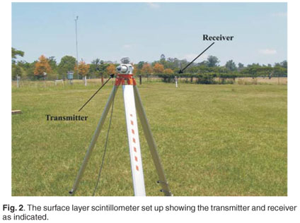By determining both the variances of the logarithm of the amplitude of the two beams, , and the covariance of the two beams, , l_o and can be obtained.⁶⁶ At the receiver, usually located 50 m to 250 m away from the transmitter, the two beams reach two separate detectors. The SLS set up is shown (Fig. 2) with a close-up of the transmitter, receiver, junction box and signal processing unit of the SLS (Fig. 3).

 

 

 

 

The covariance of the logarithm of the amplitude of the received radiation is given by:¹⁰

Equation 15 is valid for < 0.3, corresponding to weak scattering. If the scattering is not weak, then the measured is less than that determined from Equation 15 and saturation is said to occur.⁷⁶ Due to this fact, the maximum path length for the SLS is usually limited to 250 m. To overcome the saturation problem, which limits the SLS measurements to a beam path distance of 250 m, the beam path length should be decreased or beam height position increased.^3,60 Otherwise a LAS would be the option for obtaining H over longer path lengths, e.g. 5 km to 10 km.⁷⁷

The functional dependence of the covariance in Equation 15 includes two wave numbers – the optical wave number K (m^–1) for the SLS beam, where K = 2π/λ, and where λ = 670 nm for the SLS and wave number defined as κ = 2π/l, corresponding to the spectrum of eddy sizes that the beam encounters where l is eddy size. The functional dependence of Equation 15 also includes the function Φ_n(κ) corresponding to the three-dimensional spectrum of refractive index inhomogeneities caused by the interaction of changes in air temperature with refractive index, SLS beam displacement distance d_SLS, two Bessel functions J_o and J₁ of the first kind, r the distance along the beam measured from the transmitter with L_beam corresponding to the beam path length, and D_SLS the aperture diameter of the scintillometer detectors. As presented by Lawrence and Strohbehn⁷⁸ and pointed out by Thiermann and Grassl¹⁰, substituting d_SLS = 0 m corresponding to a single beam into Equation 15, provides the expression for the variances at each of the single detector pairs.