Services on Demand
Article
Indicators
Related links
-
 Cited by Google
 -
 Similars in Google
Share
South African Journal of Science
On-line version ISSN 1996-7489
Print version ISSN 0038-2353
S. Afr. j. sci. vol.105 n.1-2 Pretoria Jan./Feb. 2009
RESEARCH ARTICLES
Agriculture production's sensitivity to changes in climate in South Africa
James BlignautI, *; Liza UeckermannII; James AronsonIII
IDepartment of Economics, University of Pretoria, Pretoria 0002
IICompetition Commission, New Zealand
IIIRestoration Ecology Group, CEFE (CNRS–UMR 5175), Montpellier, France, and Missouri Botanical Garden (U.S.A.)
ABSTRACT
South Africa in general has been approximately 2% hotter and at least 6% drier over the ten years between 1997 and 2006 compared to the 1970s. The use of water has also increased greatly over this same period. By 2000, 98.6% of that year's surface water yield and 41% of the annual utilisable potential of groundwater was allocated to use. Irrigation agriculture, comprising 60% of total consumption, is by far the largest single consumer of water. Given these climatic and water use changes as a backdrop, we employed a panel data econometric model to estimate how sensitive the nation's agriculture may be to changes in rainfall. Net agricultural income in the provinces, contributing 10% or more to total production of both field crops and horticulture, is likely to be negatively affected by a decline in rainfall, especially rain-fed agriculture. For the country as a whole, each 1% decline in rainfall is likely to lead to a 1.1% decline in the production of maize (a summer grain) and a 0.5% decline in winter wheat. These results are discussed with respect to both established and emerging farmers, and the type of agriculture that should be favoured or phased out in different parts of the country, in view of current and projected trends in climate, increasing water use, and declining water availability.
Key words: agriculture production, rainfall, drought, climate change, water scarcity
Introduction
This study focused on the impact of changes in climatic conditions on agriculture: it is motivated by the fact that agriculture is the mainstay of rural economies in South Africa, and indeed throughout much of Africa. Agriculture's importance cannot be overemphasised from a food security perspective, or from its vital role in assisting the country to enhance and maintain political stability through successful land reform. Understanding changes in agriculture already taking place, or likely to take place in the near future, in response to climate change is therefore of utmost importance.
To map the historic changes in rainfall and temperature with changes in agriculture production in South Africa we were constrained to using existing provincial data, rather than biome-level data, which would have been preferable, but were unavailable. In addition, we had to limit ourselves to the period for which relevant data were available, i.e. from 1970 onwards. This of course affects the predictive powers of the models. Notwithstanding these limitations, some valuable insights were gained as to the relationships, and the challenges ahead, concerning the links between climate and agriculture.
We first consider recent changes in climatic conditions in South Africa's nine provinces, and then discuss the use of water based on a panel data econometric analysis of the relationship between rainfall and various components of agricultural production. We conclude with an assessment of the impact of rainfall specifically on field crops, as they are most likely to be adversely affected by sudden or gradual changes in climatic conditions.
Changes in climatic conditions
It is widely assumed that ongoing changes in climatic conditions will have an adverse effect on agricultural production in Africa.1–3 While the impact of climate change is felt by farmers predominantly through changes in the timing, frequency and intensity of rainfall events, and in the distribution of these events within a season of growth, most macroeconomic and agricultural production data are only available as annual averages. Yet annual numbers and averages for level of, or changes in, temperature and rainfall do not provide an adequate indication of the impact of such variations from the mean on a specific farm. Given this limitation, it should be noted that this study was not an investigation into climate change per se, even though we did analyse and discuss the data used in determining the impact of changes in climate on agriculture. A further limiting factor is that, when dealing with annual numbers, one is strictly speaking not dealing with drought as defined by McKee,4 who indicated that a drought occurs when the Standardised Precipitation Index over 12 months is continuously negative and reaches a value of –1 or less. We therefore did not consider the impact of individual drought events on agriculture, but rather the gradual drying trend on agricultural production as a whole. Our aim was to analyse the available data to examine whether changes in the variance from the mean for rainfall and temperature had indeed occurred.
Materials and methods
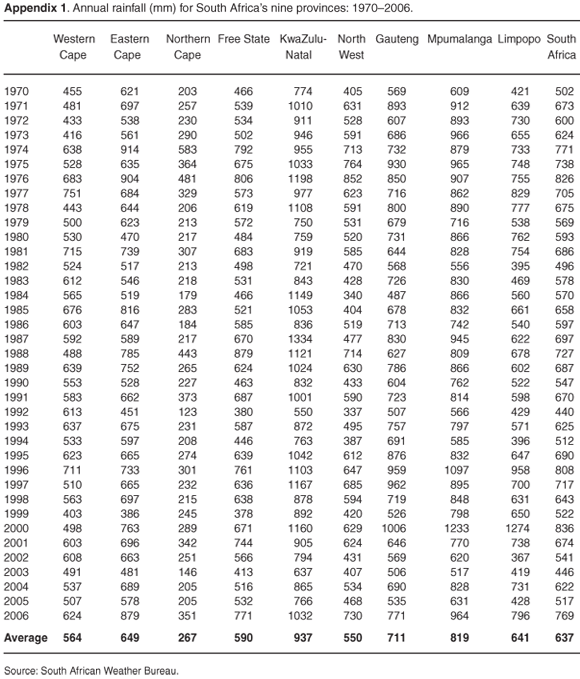
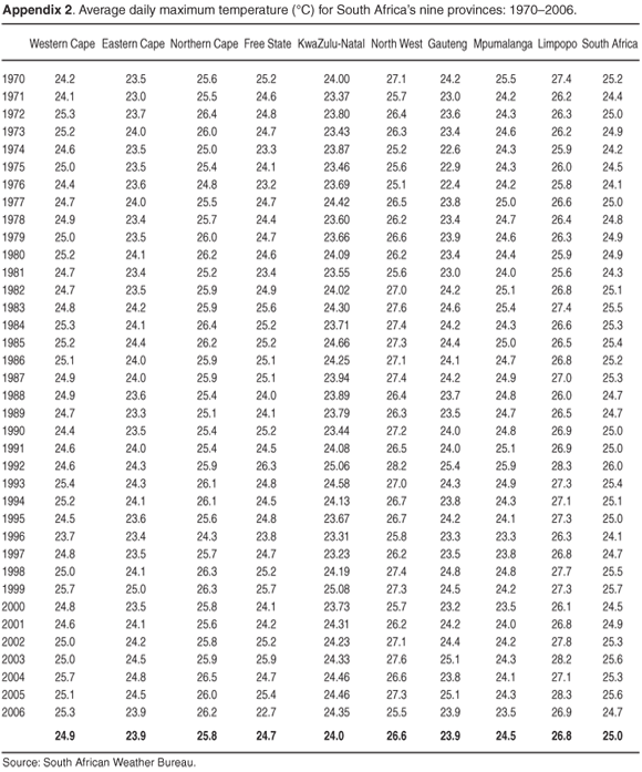
To address the broad-scale impact of climate change on agriculture, we considered rainfall and temperature data from 1970 to the present for South Africa's nine provinces. For rainfall (in mm), the annual sum of the provincial monthly average was used (Appendix 1 online). The data received were, in all cases, provided in a ready-to-use format and were not manipulated in any way. The temperature data (Appendix 2 online) consist of the annual averages of the daily maximum temperatures, in either two or three towns or cities per province. In general, daily minimum temperatures are considered a better indicator of climate change per se, but here we use daily maximum temperatures since it is these changes that are likely to have an impact on agriculture production in South Africa. The data received consisted of monthly averages of the daily maxima and, from these, we computed the annual averages.
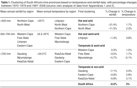
First, the nine provinces of South Africa were clustered together in four broad climatic areas in terms of their average rainfall and temperature data (Table 1). Thereafter, we calculated the changes in the average rainfall and temperature, and the changes in the variance from the mean and the covariance (Table 2). This summary contains the results for the nine provinces for the periods 1970–1979 and 1997–2006, as well as 1970–1989 and 1990–2006. The data set was split into these four separate time periods to ascertain whether there are distinct differences between the levels of rainfall and temperature among the various periods, and how weather patterns may have changed.
Results
Temperature
Several observations can be made from the results displayed in Tables 1 and 2. With the exception of a temperature decline at Mpumalanga, all the other areas showed a considerable increase—in places as much as 4%. For South Africa as a whole, the last 10 years have been on average 0.5°C—or 2%—hotter than the 1970s. The variance increased during the same period, implying that changes in temperature became less predictable, but were consistently higher in absolute terms and increased steadily over the entire period studied.
Rainfall
All but one of the nine provinces received progressively less rainfall since 1970. The exception was the Western Cape, which, on average, received consistent annual rainfall over the entire study period (Table 1). The Northern Cape and the North West provinces have in general been the most affected, both in terms of percentage change (Table 1) and absolute change (Table 2). South Africa as a whole received on average 40 mm less rain per annum over the last 10 years than during the 1970s, which means 6% less average rainfall. However, the deviation from the mean for all the hot and arid areas was less during the last ten years than during the 1970s. The variance from the mean has increased for other less arid areas, indicating increasing unpredictability and occurrence of extreme events.
In sum, South Africa has been hotter during the last 10 years compared to the first 10 years of the study period, and with more variation from the mean. Additionally, average annual rainfall was less during the last decade than during the 1970s. The variance around these lower rainfall numbers is declining for the two westernmost provinces, implying more predictability at low and declining levels of rainfall for the hottest, most arid regions. Variance, however, is increasing for the other areas, implying increasing unpredictability.
Covariance of rainfall and temperature
The relationship between rainfall and temperature was analysed using ANOVA for the individual provinces of South Africa, yielding the results shown in Table 2 and Fig. 1. For both periods studied and for all areas, the covariance of rainfall and temperature was very significantly negative (P < 0.001) for most provinces. Indeed, with the exception of the arid areas, the covariance observed between temperature and rainfall has actually become stronger over the last decade: the hotter it gets, the less rainfall there is in all regions. Should the evidence produced here signal a lasting trend, then the prevailing adverse climatic conditions are likely to persist and possibly deteriorate further. In the next section we will consider how changing climate, especially reduction in rainfall, may affect agriculture.
Water use in agriculture in South Africa
Given that South Africa, overall, is getting hotter and drier, the question is, how big is the buffer? How much surplus water does South Africa have, who is using it, and can the trend be changed in view of the declining supply? The South African Department of Water Affairs and Forestry5 estimates that in 2000 South Africa had a total reliable surface water supply of 13 226 million m3. In the same year, the nation used 13 041 million m3, leaving a surplus of only 186 million m3, or 1.4% of the supply (at 98% assurance of supply) for that year. Additionally, 12 of the country's 19 water catchments reported water deficits, which were only partially offset by an intricate system of inter-basin water transfer schemes. These statistics are supported by the water resource accounts, produced by Statistics South Africa.6 In theory, as the remaining annual supply of a vital natural resource approaches zero—crossing clearly identifiable thresholds of scarcity—the marginal value of that resource approaches infinity.7 This implies that the economic value of the last 1.4% of unutilised water resource is very high, far exceeding that of the prevailing bulk water tariff. Matters are complicated by the fact that, as water supply is annually recharged through precipitation, it does not imply that only 1.4% is available into perpetuity, but rather that for the year 2000, specifically, only 1.4% of the water supply was unallocated or not used. This implies that should the water demand grow by more than 1.4%, the only way to accommodate such growth is by reducing water use in some of the currently water-intensive sectors, which in turn implies that some tough decisions have to be made.
Moreover, the meagre water reserve mentioned above includes the water imported from neighbouring Lesotho. Unutilised domestic sources of water are limited to two river catchments in the ecologically-sensitive and relatively undeveloped Eastern Cape province. Water-supply constraints are therefore an issue with unparalleled economic development implications. Further supply options are limited, but include further water importation from Lesotho, and, additionally from the distant Congo River, and/or desalination of seawater. All three of these options are costly and capital intensive and their implementation would have a significant effect on water tariffs with the result of making drinking water less accessible to those who are most in need. In other words, only 1.4% of South Africa's water yield is currently available to address the demands of the poor, most of whom who do not have any access to potable piped water currently. But has the market reacted to these changes? Have water use extraction and allocation trends already changed?
Surface water use
Irrigation agriculture is by far the largest single surface water user, consuming 60%, with agriculture in general consuming 65% of total available water.6 Use of surface water for irrigation has also increased steadily from 7630 million m3 in 1995 to 7921 million m3 in 2000, an increase of 291 million m3, or 4%. This use represents 160% of the total water surplus remaining at the end of 2000. The official water use for 2005 has not yet been released, but if the volume of water used for irrigation increased by the same margin, without any compensatory reduction in water use by other sectors having taken place, there must have been a deficit for the country as a whole. Furthermore, the total increase in water consumption for all sectors from 1995 to 2000 was 348 million m3, which implies that irrigated farming's share of the increase was 84%.
Groundwater use
Surface water use is increasing rapidly, with no signs of a decline in use in any sector. Use of groundwater is increasing rapidly as well.8,9 Vegter8 estimates that by 1999 there were approximately 1.1 million water boreholes in the country, compared to only 225 000 recorded on the National Groundwater Database. From drilling data and agricultural records, Vegter8 calculates that the groundwater use in 1999 was about 3360 million m3 per year and is increasing at, on average, approximately 3.4% per year. The estimated use at the end of 2001 was approximately 3850 million m3, or 49% of the surface water usage. The exploitable groundwater usage for 2000 is estimated6 at 9500 million m3, which implies that groundwater usage at that stage was about 41% of the potential. This allows room for some further development, but clearly the surplus is dwindling fast. In fact, water abstraction of both surface and groundwater has increased so quickly in recent years, being used primarily to drive the development of agriculture, mainly in the horticulture and animal production sectors.
Water: The limiting factor
Water is therefore one of the main, if not the, limiting resource upon which intelligent, sustainable economic investments should be concentrated.10–13 Water use, given the supply constraints, cannot continue to grow at current rates. This situation is exacerbated by the likely decline in the water availability due to changes in climatic conditions, and socio-economic and demographic pressure to increase the use of potable water for domestic use and to allocate water to higher value added industries. Another complicating factor is the plausible introduction of a wide-scale biofuel programme and its plausible impact on future water demand.
Quantifying rainfall's contribution to agriculture
Model
We developed a Seemingly Unrelated Regression (SUR) model (Appendix 3 online), using a three-dimensional panel data set, to quantify the contribution of rainfall to agriculture. Hsiao14 defines a panel data set as one that follows a given sample of individuals—provinces in this case—over time, and thus provides multiple observations on each individual in the sample. Here the dimensions are time, geographic area (nine provinces), and a series of variables. From a modelling perspective, panel data is therefore very powerful, as it combines regular time-series and cross-sectional regressions, and has numerous other advantages.14–16
Data
We gathered data for each province over the period 1970– 2006, for gross income from agriculture (subdivided into three sectors: field crops, horticulture, and animal production), expenditure on intermediate goods and services, labour and other expenditures, net income, and contribution to GDP. It was not possible to allocate the cost items to specific agricultural sectors since no method to do so exists. To estimate provincial shares, we used data from unpublished sources, mostly from the archives of the National Department of Agriculture (NDA) in Pretoria, including agriculture surveys from 1971, 1973, 1975, 1978, 1981, 1983, 1988, 1993, 1995, and 2002. Interpolation was used to construct a complete time series for all the provincial shares for which no data exist. Most importantly, all nominal values were deflated using relevant price indices obtained from the NDA. Gross income in constant prices was plotted against the volume of production index revealing the same trend and slope—a clear indication that an appropriate deflator was used.
Results
The results from the SUR model for field crops, horticulture, and animal production are summarised in Table 3. The model does not allow for variation in the slope of the net income function among regions, but the variation in the intercept of the regions through the SUR model specification has been permitted. The Adjusted R-squared values of 0.92 and higher indicate that the SUR models represent a good fit of the data, supported by significant F-statistics of 42 281 (field crops), 6 820 (horticulture), and 61 431 (animal production), respectively. The coefficients of the interaction variables are almost all significant at the one per cent level (P < 0.01).
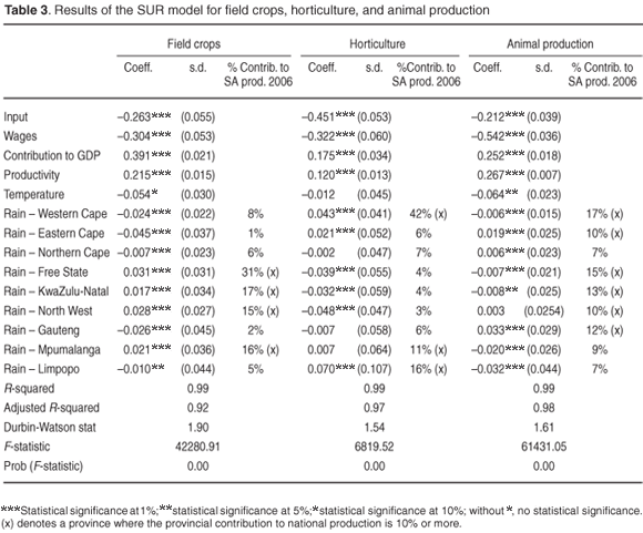
Based on the estimations obtained in Table 3, the net income function (Equation 1) can be specified for field crops, horticulture, and animal production for each province.
Field crops:
YFCit* = Ci – 0.26inputit – 0.30wagesit + 0.39conit + 0.21Prod – 0.05tempiti ,
where Ci = αirainit (province)
Horticulture:
YHit* = Ci – 0.45inputit – 0.32wagesit + 0.18conit +0.12Prod – 0.01tempiti ,
where Ci = αirainit(province)
Animal production:
YAit* = Ci – 0.21inputit – 0.54wagesit + 0.25conit + 0.27Prod – 0.06tempiti ,
where Ci = αirainit (province)
Since these net income functions were estimated in log terms, the coefficients can be interpreted as percentage changes, implying, for example, that a 1% increase in expenditure on intermediate goods and services will lead to a decline in net income of 0.26% for field crops.
Discussion
Gross farm income (gross revenue or turnover) in real terms (constant 2000 prices) over the entire period has grown only marginally, with the exception of the Western Cape. Here the growth in viticulture contributed significantly to the growth in the sector over the initial few years of the study period. This steady growth has been offset by a rapid rise in production costs in all provinces leading to a declining net income (revenue minus cost), which is currently at worrisomely low levels. Within the context of this paper, this suggests that first, increases in gross income occurred despite increasingly adverse climatic conditions; and, second, that the decline in net income is predominantly the result of an increase in input cost. The evidence from Table 3 supports this conclusion. The size of the coefficients of the costs, productivity, and sector size for each of the three agriculture sectors is far bigger than that of either rainfall or temperature. Third, this suggests that the increase in gross production could only be attained through the relative increase in the use of financial capital to attain this growth in gross income, but at a significant financial cost. The use of capital, as indicated by the formation of fixed capital (or investment), has remained constant in real terms since 1970 at approximately R6 000 million,17 but employment has declined from more than 1.6 million in 1970 to just over 600 000 in 2005—or about 36% of the 1970 level.4,18 This trend runs counter to the steady growth in both population and unemployment, and therefore signals a clear shift towards more capital-intensive agriculture. Fourth, the increase in capital intensification, also illustrated by the size of the coefficient for input costs, coincides with an increase in irrigation as discussed above. This suggests that, if it were not for irrigation, the growth in gross income might have been much less, but that such expansion and intensification have important financial costs, which are rising much faster than the value of the product. Fifth, temperature is indeed negatively correlated with net farm income for the three sectors, but has a very small coefficient, and is not statistically significant for horticulture production. However, the results from Table 3, with regard to rainfall, reveal a positive correlation between rainfall and net income for field crops and horticulture, for each of the provinces that produce more than 10% of the national output—indicated with an 'x' in Table 3. These data are important from a food security perspective.
For animal production, the relationship is less clear. Animal production includes poultry farming—which is currently the single largest agricultural sector in the country—and cattle farming for beef. Beef production in South Africa today is largely feedlot-based, though most of the animals originate from cattle farmers. In other words, calves are free-ranging until they are about nine months old, when they are auctioned to feedlot owners. Cattle, however, are counted as part of animal production only after being slaughtered. Therefore, there is no direct link between rainfall and animal production, as both poultry and beef production use abstracted water. For beef production, this can lead to erroneous conclusions, as the productivity of free-range cattle husbandry is adversely affected by any reduction in rainfall. This degree of dependence is not reflected in the data used here, as livestock sales are not counted as animal production. In 2004, so-called subsistence farmers owned 5.6 million head of cattle, i.e. 41% of the national total of 13.8 million.19 These individuals are extremely vulnerable to changes in climate and, given the small scale of their operations and the limited access they have to open markets, the value of their animal production is not captured adequately in a macro-economic data set, such as the one used here. This is also a group of farmers which has not yet been integrated into the formal agriculture sector, despite governmental pressure to do so. Adverse climatic conditions are likely to make this process more difficult to accomplish.
We have seen that rainfall is significant to the dominant horticulture production areas such as the Western Cape, where viticulture plays a major role. Horticulture, like animal production, makes extensive use of irrigation that temporarily offsets any sudden decline in rainfall. In contrast, dry-land agriculture, especially involving field crops, cannot make use of irrigation and is therefore much more vulnerable to changes in climatic conditions than horticulture and animal husbandry. Given both the importance of rainfall for field crop production, and that field crop production is likely to be most affected by any adverse changes—sudden or gradual—in climatic conditions, we conclude our analysis by considering the relationship between rainfall and field crop production in more detail.
Production of field crops and rainfall
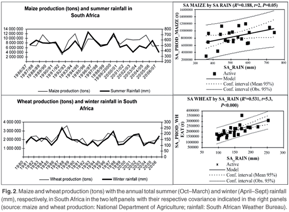
There is a remarkable correlation between rainfall and crop production, whether summer (e.g. maize) or winter crop (e.g. wheat), as seen in Fig. 2, where we distinguish winter rainfall (April–September) from summer rainfall (October–March). We use maize and wheat as proxies for all seasonal field crops to demonstrate the link between rainfall and crop output.
To determine the specific relationships between rainfall and crop production for these respective crops, for each area, an elementary equation was used:
% change in productioni, j = % change in rainfalli ,
where i represents each province and j a given crop (Table 4). As the function was estimated as a percentage change, coefficients indicate that for every 1% change in rainfall, the expected change in gross production is 'x'. For all the provinces contributing approximately 20% or more to national production for either maize or wheat—the Free State (40%), Mpumalanga (21%), and the North West (18%) for maize, and the Western Cape (35%) and the Free State (37%) for wheat—highly statistically-significant relationships (P < 0.0001) were found between crop production and rainfall. Maize production is generally more sensitive to changes in rainfall than wheat production, as indicated by the respective sizes of the coefficients. Alarmingly, a 1% change in rainfall should lead to more than a 1% change in maize production. This does not augur well for provinces such as the Free State, the North West, and the Western Cape, as these provinces were considerably warmer from 1997 to 2006 than in the three preceding decades (Table 2). Additionally, there is a strong negative relationship between temperature and rainfall, especially in the two former provinces. Should it become still warmer in the future and rainfall continue to decrease, then the three major maize and wheat production areas of the country will be susceptible to marked reductions in crop production.

Conclusion
South Africa, on average, has been hotter and drier during the last 10 years than during the 1970s. If this represents future climatic trends this has major implications for South African agriculture. Notably, there is very little scope for expansion of irrigation, given the limited supply of non-saline water and pressing socio-economic needs. This scenario implies that farmers are likely to rely increasingly on water-saving techniques that may drive up costs even further, in a sector that has a small net income margin and which is already facing rapid cost rises. This is likely to make it increasingly difficult for emerging farmers to enter the sector, despite the official national policy to help them. In addition, there likely will be significant impacts on food security, which is already under pressure.
Furthermore, there is a statistically-significant positive correlation between the production of field crops and horticulture in all the provinces that contribute more than 10% of the national supply. Given trends of declining rainfall and increasing average temperature, and the statistically-significant negative relationship between these two variables, this implies that both field crop production and horticulture are extremely vulnerable, especially rain-fed field crops. A 1% decline in rainfall is likely to lead to a decline in maize production of 1.16% and a decline in wheat production of 0.5%. Such a decline in rainfall is also likely to lead to a decline in net income in the most productive provinces.
As we have seen, only 1.4% of South Africa's water yield is currently available to address the demands of the poor, most of whom currently have no access to potable piped water. These 15 million people, who comprise 35% of the population,20 are obliged to find and physically carry water to their homes and their livestock on a daily basis—clearly not a tenable situation.
Even under pre-industrial conditions, ecological systems, including agrosystems, were subject to influences from extreme events and global forcing factors, such as new markets or the collapse of old ones. In the context of recent massively accelerating anthropogenic climate changes, we need to adapt our ways of thinking, acting, farming, and managing vital resources, particularly water.
The authors are grateful to Dirk Blignaut of the National Department of Agriculture and Benedict Libanda and Giotseope Mmopelwa for assistance in compiling the database. We also thank Colleen Seymour and three anonymous reviewers for helpful comments on the manuscript.
1. Maddison D., Manley M. and Kurukulasuriya P. (2007). The Impact of Climate Change on African Agriculture: A Ricardian Approach. Policy Research Working Paper 4306, The World Bank, Washington D.C. [ Links ]
2. Stern N. (2006). The Economics of Climate Change. Cambridge University Press, Cambridge. [ Links ]
3. Kurukulasuriya P., Mendelsohn R., Hassan R., Benhin J., Deressa T., Diop M., Mohamed Eid H., Fosu K., Gbetibouo G., Jain S., Mahamadou A., Mano R., Kabubo-Mariara J., El-Marsafawy S., Molua E., Ouda S., Ouedraogo M., Se'ne I., Maddison D., Niggol Seo S. and Dinar A. (2006). Will African agriculture survive climate change? World Bank Econ. Rev. 20, 367–388. [ Links ]
4. McKee T.B., Doesken N.J. and Kleist J. (1993). The relationship of drought frequency and duration of time scales. In Eighth Conference on Applied Climatology, American Meteorological Society, Anaheim CA, pp. 179–186. [ Links ]
5. DWAF (Department of Water Affairs and Forestry) (2004). National Water Resource Strategy. DWAF, Pretoria. [ Links ]
6. SSA (Statistics South Africa) (2006). Water Resource Accounts for South Africa: 1995 & 2000. SSA, Pretoria. [ Links ]
7. Farley J. and Gaddis E. (2007). Restoring natural capital: an ecological economics assessment. In Restoring Natural Capital: Science, Business and Practice, eds J. Aronson, S. Milton and J.N. Blignaut, pp. 17–27. Island Press, Washington D.C. [ Links ]
8. Vegter J.R. (2001). Groundwater Development in South Africa and An Introduction to the Hydrogeology of the Groundwater Regions. Water Research Commission (WRC) document TT 134/00. WRC, Pretoria. [ Links ]
9. Botha F.S. (2005). A proposed method to implement a groundwater resource information project (GRIP) in rural communities, South Africa. M.Sc. thesis, University of the Free State, Bloemfontein. [ Links ]
10. Scholes R. (2001). Global Terrestrial Observing System: Regional Implementation Plan for Southern Africa. GTOS-21. CSIR, South Africa. [ Links ]
11. Daly H.E. and Farley J. (2004). Ecological Economics. Island Press, Washington D.C. [ Links ]
12. Aronson J., Blignaut J.N., Milton S.J. and Clewell A.F. (2006). Natural capital: the limiting factor. Ecol. Eng. 28, 1–5. [ Links ]
13. Farley J. and Daly H.E. (2006). Natural capital: the limiting factor: a reply to Aronson, Blignaut, Milton and Clewell. Ecol. Eng. 28, 6–10. [ Links ]
14. Hsiao C. (2003). Analysis of Panel Data. Cambridge University Press, Cambridge. [ Links ]
15. Zeller A. (1962). An efficient method of estimating seemingly unrelated regression and test for aggregation bias. J. Am. Stat. Assoc. 57, 348–368. [ Links ]
16. Baltagi B. (1980). On seemingly related regressions with error components. Econometrica 48, 1547–1551. [ Links ]
17. South African Reserve Bank. Quarterly Bulletin. Various issues. [ Links ]
18. NDA (National Department of Agriculture) (2007). Abstract of Agriculture Statistics. NDA, Pretoria. [ Links ]
19. NDA (National Department of Agriculture) (2004). Estimated Livestock Number. NDA, Pretoria. [ Links ]
20. SSA (Statistics South Africa) (2002). South African Statistic 2002. SSA, Pretoria. [ Links ]
21. Avery R. (1977). Error components and seemingly unrelated regressions. Econometrica 45, 199–209. [ Links ]
22. Bhargava A., Franzini L. and Narendranathan W. (1982). Serial correlation and the fixed effects model. Rev. Econ. Stud. 4, 533–549. [ Links ]
Received 3 June 2008. Accepted 12 February 2009.
This article is accompanied by supplementary material online at www.sajs.co.za
* Author for correspondence: james@jabenzi.co.za.
Supplementary material to:
Blignaut J., Ueckermann L. and Aronson J. (2009). Agriculture production's sensitivity to changes in climate in South Africa. S. Afr. J. Sci. 105, 61–68.
Appendix 3. Explaining the SUR mode.
We employed the SUR model with a one-way error component, which allows cross-section heterogeneity in the error term; i.e. uit = µi + νit. On the other hand, a two-way error component model allows cross-section heterogeneity, as well as time effects; i.e. uit = µi + λt + νit. We adopt Avery's21 approach, as presented in Baltagi,16 to explain a SUR model in a panel context. The SUR model has a set of M equations:

where yj is NT × 1; Zj is NT ×  and the residuals from each equation with random vectors of Zu = (In ⊗ lT); µ'j = (µ1j,...µNj) and ν'j = (ν11j,.....,ν1Tj,....,νN1j,...,νNTj).
In addition, µ ~ (0, Σµ ⊗ IN) and ν ~ (0, Σν ⊗ INT). From Equation 1, it follows that each different equation has the same standard variance-covariance matrix. However, within a panel SUR model, there are additional cross-equation variance components. Accordingly, Avery21 defined a variance-covariance matrix that is not equation specific:

where µ' = (µ1',....,µ'M) is a 1 × MTN vector of disturbances with µj and Σu =  , as well as, Σν =
  are both M × M matrices. Replacing JT with T
 and IT by ET +
  provides the following:

It is then possible to estimate Equation 3 in a panel context, by replacing the matrix of disturbances for all M equations by OLS (Ordinary Least Squares) residuals21 or within-type residuals.16 To quantify the impact of rainfall's contribution to agriculture, we used an econometric model custom-made for this purpose. A net income function was estimated and fitted to the data with a cross-section SUR model for field crops, horticulture and animal production, respectively.

where Yi = net income for province i; Inputi = expenditure on intermediary goods and services for province i; Wagesi = wages, interest, and other sundry expenses for province i; Coni = proportional contribution to GDP for province i; Prodi = an index of gross income for province i; Tempi = temperature for province i; Raini = rainfall for province i.
We compiled three separate models for each agricultural product, namely FC (field crops), H (horticulture), and AP (animal production), respectively, where each model contained the above independent variables per region/province and the dependent variable, i.e. the net income per province, for the respective agricultural product. After the initial round of estimating the net income function—for FC, H, or AP respectively—for each of the nine provinces, using the one-way error SUR model, two problems were encountered—heteroscedasticity and serial correlation—both of which had to be corrected, as we will now explain.
Heteroscedasticity
The standard SUR one-way error component model assumes that the regression disturbances are homoscedastic, when the same variance across time and individuals occurs. This may be a restrictive assumption for panels and agricultural type data, where the cross-sectional units may be varying in size and, as a result, may exhibit different variations.22 Therefore, to correct for the potential problem of heteroscedasticity, White's cross-section heteroscedastic structure was specified in all the models, to ensure consistency and efficiency of the estimators.
Serial correlation
Another problem within the standard SUR one-way error component model is the assumption that the only correlation over time is due to the presence of the same individual effect across the panel.22 This assumption ignores the effect of an unobserved shock that took place in the current period on the following periods, causing inefficient estimates of regression coefficients and biased standard errors. In an attempt to test for serial correlation, we employed the Durbin-Watson (DW) test and Lagrange Multiplier (LM) test. In particular, the LM-test is based on the test for random effects and serial correlation, where the null hypothesis is H0 =  = 0;λ = 0 or H0 =
  = 0; ρ= 0. To construct the test, the following specification was used:

where  (
( = 0);
= 0);  (ρ = 0) and
  is OLS residuals.
The null hypothesis is rejected if the LM statistic exceeds the  (= 5.99) value. Moreover, Bhargava et al.22 outlined the DW-test, with the null and alternative hypotheses as H0: ρ = 0 and HA:|ρ|<1. These authors defined the test statistic as:

with νit is the within residuals.
The critical values in Table II from Bhargava et al.22 form the decision basis for this test. With the application of the DW and LM-tests, the results in Table A3.1 indicate that serial correlation was present.

To correct for serial correlation, we estimate rho-values for each model and each province to account for the heterogeneity across the provinces. The rho-values reported in Table A3.2 confirm the presence of serial correlation in both models along with heterogeneity across the regions.
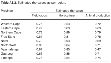
To correct for the serial correlation problem, the rho-values shown in Table A3.2 are used to transform the correlated errors into uncorrelated errors, based on a Prais-Winston transformation approach for each province. The DW- and LM-tests are performed again to determine whether serial correlation is still present in the models. Table A3.3 shows that the serial correlation problem has been addressed.
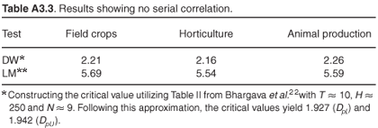
It is important to note that, with the correction for serial correlation, the sample size changed from the period 1971 to 2006, since observations have been lost through differentiation in the data transformation process. Given that the major data problems have been rectified, the final SUR models can now be presented. The results of each model are shown separately, first the field crops model, then the animal production model, and, last, the horticulture model.


