


Services on Demand
Article
 English (pdf)
 Article in xml format
 Article references
Indicators

Related links
-
 Cited by Google
 -
 Similars in Google
Share

 Permalink
South African Journal of Science
On-line version ISSN 1996-7489
Print version ISSN 0038-2353
S. Afr. j. sci. vol.104 n.5-6 Pretoria May./Jun. 2008
BIOLOGICAL MODELLING
Computer construction of species richness maps: testing a new type of multifractal algorithm
Edith PerrierI, II; Henri LaurieII, *
IIRD, UR 079 GEODES, 32 Avenue H. Varagnat, Bondy 93143 cedex, France
IIDepartment of Mathematics and Applied Mathematics, University of Cape Town, Rondebosch 7701, South Africa
ABSTRACT
We show how a new theoretical multifractal model provides means to generate virtual maps of highly variable spatial distributions of species richness. It should allow for various computer experiments in landscape ecology and the study of biodiversity. In this paper, the explicit distribution of species-representative individuals over a large range of scale leads to an original algorithm for the estimation of the Renyi dimensions of a multifractal measure. The method is successfully tested for simulated (S, A) data sets, where the variableS is simply the number of species found in a given domain of area A. This easy tool will help to characterize the spatial variability of multiscale density distributions in many fields, requiring only randomly sampled data at different locations and scales.
Introduction
Multifractal theory has been used in many fields to characterize heterogeneous distributions of measures in space and across scales (climatology,1 oceanography,2 geology and hydrology,3 and the social sciences4). From the theoretical point of view,5 a multifractal measure6 can be seen as an abstract concept, generalizing mathematical theories of measure to non-Euclidean cases involving non-integer dimensions, in a manner similar to the development of fractals. Multifractals are not fractals, though the concepts are related. Multifractal studies are concerned with scaling measures whose numerical values vary according to location and scale within a given domain. The sub-domain where the measure is defined and non-zero is called the 'support' of the measure. An example may help to clarify the term: the range of a species is the support of its density—that is, all points where the density is not zero. Fractal approaches deal with scaling properties of geometrical objects. As such, the support of a measure may be fractal or Euclidean. For example, a square embedded in two-dimensional space is a Euclidean object whereas multiscale lacunar objects such as the Sierpinski gasket are non-Euclidean and are classical examples of non-Euclidean fractal geometrical sets.7 A fractal object may be characterized by its fractal dimension D, whereas a multifractal object instead needs to be characterized by a function such as its spectrum of Renyi dimensions D(q). These dimensions describe for each moment of order q the scaling law of the measure densities. The Renyi dimension associated with the moment of order 0, i.e. D(0), is equal to the dimension of the support. If the support is Euclidean, then D(0) = d, the Euclidean dimension, whereas if the support is fractal of dimension D, then D(0) = D < d.
In many examples, multifractal theory has usefully characterized heterogeneous, multiscale spatial distributions whose variations increase in a more or less self-similar way as the resolution increases. We know that many variables are unequally distributed in space (rainfall,1 river network density,3 vegetation2, human population,4 etc.), and we can surmise that zooming in will reveal increasing variability. Using multifractals, such a phenomenon can be described by a multiplicative cascade process which reproduces at each scale a self-similar pattern of the partition into poorer and richer regions. The issue of strict self-similarity of the variability increasing throughout scale is an open research question. As with fractals, the self-similar case may merely be a mathematical convenience. Deviations from self-similarity should be handled by extending the reference model in more complicated multiscale analyses or in exploratory simulations.8
For end-users, a multifractal approach can be seen as a new, constructive tool in the field of spatial statistics. It adds to the field in that the usual spatial statistics characterize data but do not furnish methods for actually realizing the spatial patterns they model. For example, it is easy to compute the variogram of a spatial variable but it is more difficult to define a theoretical variable reproducing the spatial structure of the observed variable. Multifractal models may be an idealized and simplified approach of multiscale complex spatial systems compared with more sophisticated statistical theories, but we will show in this paper that they may provide means to simulate virtual worlds having the same statistical properties as observed ones as well as promising qualitative properties.
Our illustrations will be based on the MFp1p2 model, which has been conceived to describe the spatial distribution of species.9 It is similar to a model in physics for some heterogeneous distribution of mass.10 The MFp1p2 model provides a new type of application of multifractals that clearly illustrates multifractal theory and that can be easily interpreted in terms of a self-similar multiplicative cascade of species distribution in poorer and richer parts at successive scales. It provides also the means to build actual computer models which mimic the real world.
In the first section we show how we can build computer models of species richness using an object-orientated and individual-based modelling approach to build virtual maps of the presence/absence of species at different scales. In the second section we will use the virtual maps to test a new algorithm adapted to a common case: data resulting from random sampling strategies on irregular domains.
Generating multifractal virtual species maps
The theoretical model
The MFp1p2 model conceived by Laurie and Perrier is a novel application of multifractal theory devoted to the quantification of the spatial variability of species richness. It is based on iterated bisections of the whole studied domain Ω (with a given area Amax and containing a number Smax of species) into two subdomains, where p1 represents a proportion of species present in the first subdomain, and p2 a proportion of species present in the second one (see Fig. 1). Analytical calculations have shown that this model is a perfect multifractal when the two parameters p1 and p2 (0 < p2 < p1 < 1) are constant throughout successive bisections over an infinite range of scales. It has been shown that this model explains the classical power-law SAR widely used by ecologists to characterize different types of species, because it reduces to Harte's model11 when p1 = p 2 (i.e. when no spatial variability is addressed), and that it can explain the observed spatial variability at all scales around the power-law trend as soon as p1 ≠ p2.

We show in the following section that this conceptual model can be implemented in computer simulations, which provides thereby a self-contained description of the MFp1p2 model, and more generally a straightforward illustration of multifractal theory through an illustrative example.
Individual-based modelling
To generate a computer realization of the MFp1p2 model,12 we first take advantage of an object-orientated programming style8 to deal with a hierarchical graph of embedded spatial subdomains.
We define specific types of computer objects called Classes (see boxes on this page for a simplified description of two examples of classes called Cells and Species). Each class instance is defined by its own encapsulated attributes and has access to the methods of its class. One can store further categories of information through the addition of new attributes. Each cell can store many attributes, such as links to neighbours, parent or children, which will be useful in further studies involving the simulation of dynamical processes occurring on the cell network, but in the present paper we restrict ourselves to the representation of static properties, as described later on.
| Class Cell Attributes: Space: the geographical definition. In the present version, an instance of the class Space is just a list of vertices: four vertices are used to define a rectangular domain; polygonal or more complex shapes could be used as well. Level: the level k where the cell was created in the iterative construction. nbSpecies: the number of species present in the cell. Methods: Area(): Calculation of the cell area, which can be trivial for simple types of Space. Centre(): Another geometrical calculation depending on the type of Space. Divide(): Creation of two daughter cells. |
The creation of a realization of a MFp1p2 model proceeds as follows: At the first level k = 0 in a simulation, a (root) cell is created to represent the total studied domain W, with a Space of area Amax, Ω.Level = 0, Ω.nbSpecies = Smax. Then, in a recursive way, a cell of level k uses its method Divide() to give birth to two daughter cells with Level = k + 1, and so on until the level kmax is reached (the maximum possible value for kmax depends on computer memory). Each daughter cell Space is calculated geometrically from the mother's Space characteristics. The method Divide() also calculates the number of species of each child using the two model global parameters p1 and p2, with nbSpecies = p1 × Parent.nbSpecies for the richer child and nbSpecies = p2 × Parent.nbSpecies for the poorer one [see Fig. 1(a)]. Let us note that easy extensions of the model could be introduced in the simulations by allowing the parameters p1 and p2 to vary as a function of level k, but at this stage, we will stay as close as possible to the pure multifractal approach, considering self-similarity over a finite but large range of scales. After kmax levels of bisection, the value nbSpecies of the multifractal measure has been defined in 2kmax Cell instances. We will see later on how it can be calculated in any other subset of the spatial support Ω.
| Class Species Attributes: Id: an identifying number within the whole set of considered species Display: a symbol or icon to plot a given species Methods: Occurrence(k): Calculation of the proportion of cells occupied by a given instance of species at level k. |
We aim also at building computer models of the distribution of species richness as close as possible to real data. In this context, first we have to deal with integer numbers of species rather than with possible non-integer proportions of the total number of species. Second, it would be very convenient to be able to track the distribution of each species, to compare individual species distribution and global richness as do naturalists. That is why we introduce a second type of computer objects, called Species.
Then the creation of an 'individual-based' version of the MFp1p2 model proceeds as follows. Taking advantage of the ease with which class attributes and methods can be extended, we add a new attribute to the Cell class, called ListIds, to represent an actual list of individual species Ids which are explicitly allocated by Cell.Divide() in the computer construction. As described in Fig. 1(a), knowing ListIds of the mother cell (all the ids for the root domain Ω), the species are divided into three subsets in the proportions 1 – p1, 1 – p2, p1 + p2 – 1 (suitably rounded to integers), then distributed to reach the required proportions p1 and p2 in the daughter cells, which update their own ListIds with the species they receive.
Such an 'individual-based' recursive allocation of species-representative ids from mother cells to daughter cells at each iteration k results in the generation of a set of spatial domains (the cells) of area Ai containing an integer Si number of species. If Si < 1, proportions can be replaced by probabilities for a single species to be present in one of the two daughter cells, but the simulations presented in this paper avoided this extension of the model by imposing a limited number of iterations kmax, depending on the total number of species Smax present in the initial domain Ω.
We focus on the creation of richness virtual maps to be compared with real maps. A virtual map of the domain Ω is first of all a partition of Ω into elementary cells. But a map can also be defined at each level k as the set of all cells at that level: Map(Ω, k) = {Celli, i ∈ [1,n = 2k]|Celli. Level = k}. Some examples are shown in Fig. 1(b). As regards species richness, and at a given resolution or scale defined by the value of k, we can store in the map two types of information. In Map(Ω, richness) = {Celli.Space, Celli.nbSpecies, i ∈ [1, n]}, we store only the number of species. In Map(Ω, species) = {Celli.Space,Celli.ListIds, i ∈ [1, n]}, we store the list of species ids present in each cell, as well as the other information.
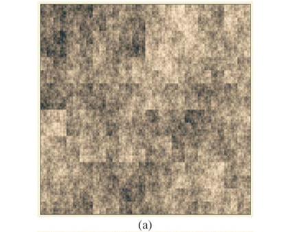
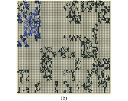
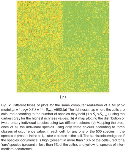
These types of format are similar to formats which can be used in Geographical Information Systems to store real maps. Figure 2 depicts examples of maps obtained using the same parameters on a square domain Ω for various properties and different types of display. In Fig. 2(a) we plot the richness map with different intensities of the grey levels according to the number of species in each cell. This map is almost equivalent to the one which would have been obtained using only theoretical proportions and without explicit allocation of individual species. Equivalence will be tested in the following section using the numerical estimation of multifractal dimensions. In Fig. 2(b) the presence/ absence of two arbitrary individual species is plotted to display the actual information stored in the simulator information. In Fig. 2(c) the presence/absence of all the individual species is plotted altogether. Because it is impossible in most cases to read a map using as many symbols as species, we used the method Occurrence(k) defined for each species to display only three types of symbols, depending on three classes of rarity/abundance over the whole simulated domain. Incidentally, this opens further possibilities of explorations by simulation to match the patterns observed in real maps.
Testing a new algorithm to calculate multifractal Renyi dimensions
The virtual maps which have been constructed have the same format as real maps. In this section, we report how we used them to generate simulated data and to investigate how multifractal dimensions can be estimated from real maps.
Theoretical Renyi dimensions
A classical way to characterize a multifractal measure consists in calculating its Reyni dimensions using partitions of the domain in N(r) boxes of linear size r. One needs the density pi of the ith box with length r, defined by pi(r) =  , where Ni is the 'mass' in the ith box.5 In the case of species richness, the M i are given by the count of species in the area represented by the ith box. The dimensions D(q) are then defined by the following equation.
It can be shown for MFp1p2 this reduces to
so in our case D(q) depends on the single parameter b =  .
.
Numerical estimations from the construction process
A difficulty arises in the calculation of D(q) from real data, as it is impossible to handle an infinite range of scales and hence mathematical limits cannot be taken. The classical method5 consists in plotting (log 
 (r), log(r)) data for a finite set of available r values (if q ≠ 1), or (if q=1), and estimating D(q) from the slope of a regression line, for example by least squares. For example, the multifractality of black and white images can be tested in this way.7 There, the measure M is the black part of the object and its mass distribution is analysed at different resolutions. The image is partitioned into boxes of size r over the available range of scales between the dimension of the image and the size of the elementary pixel at the lowest resolution. In the case of the application of the MFp1p2 model to real data, the multifractal measure is the species richness density, and the data are integer counts of the number of species S(r) present in a box of size r.
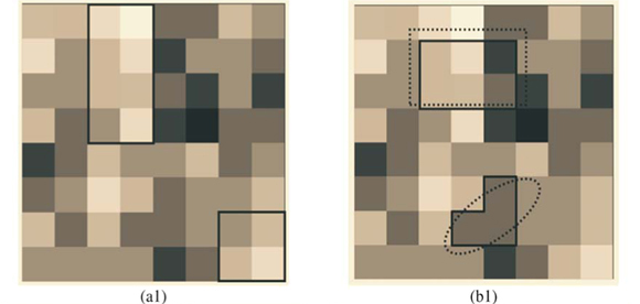
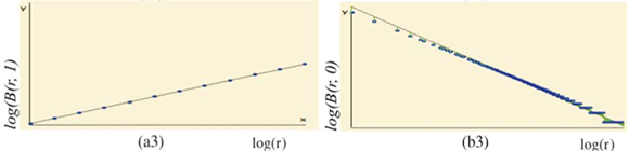
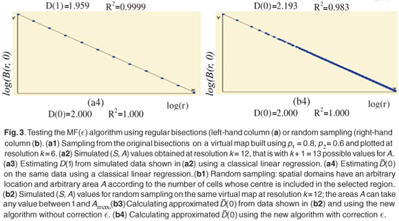
We first checked the reliability of the virtual maps, as regards the implementation of a multifractal object, by estimating their D(q) dimensions as follows. The map was partitioned in boxes selected to cover the whole map as in the theoretical approach, that is, using the N (r) = 2k rectangles of area 2kAmax and linear size r = 2- k / 2  defined at each iteration k of the hierarchical construction [Fig. 3(a1)]. We know by construction the number of species Si(r) in each rectangular cell. The calculation of local densities is straightforward: pi (r) =
  for each q ≠ 1, the plot of log (r)versus log(r) is highly linear [see Figs 3(a3) and 3(a4)] and, for any q ≠ 1, the estimation of
  (q) of D(q) from the slope of the regression line divided by (q – 1) is very close to the theoretical value given by Equation (2), namely, (0) = D(0) = 2 [Fig. 3(a4)]. Similar results hold for the special case of D(1) [Fig. 3(a3)].
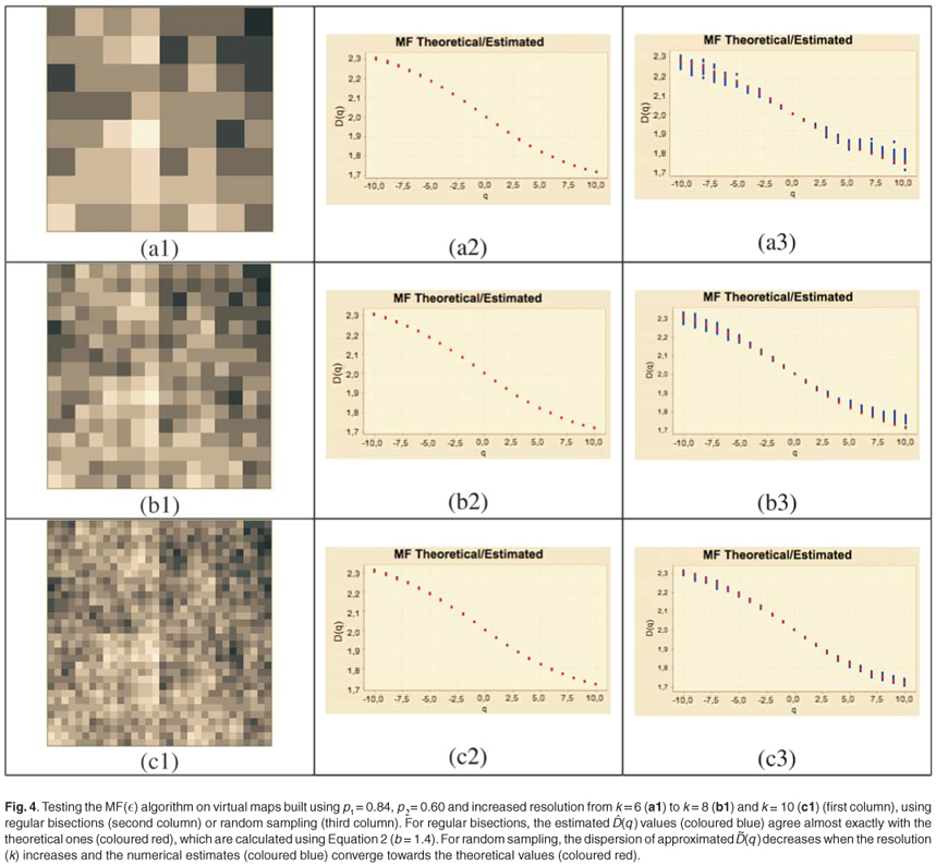
The whole spectrum of (q) values is plotted on Fig. 4 (second column) at different resolution levels. Due to the self-similarity of the construction process, only a few levels are required to get numerical estimates (q) very close to the expected theoretical ones (q) and the results are similar for low- or high-resolution data [Figs 4(a2), 4(b2) and 4(c2)].
We can conclude that the statistical estimation (q) ≈ D(q) over a finite range of scales is valid and that our richness virtual maps are actual realizations of the multifractal model based on successive bisections.
Approximate Renyi dimensions for partial and random data sets
In the real world, we do not have bisections given from a construction process. Instead, we have geographical maps on irregular domains. And richness data are often given on arbitrary sub-domains as a list of (S, A) values, where S is the number of species counted on a sub-domain of area A. Such richness data lead to the construction of Species Area Relationships (SARs), which play an important role in theoretical and applied ecology.11 The issue we address here is: how to estimate the D(q) dimensions from real data sets, in order to assess quantitatively the multifractality of species richness distribution. It has been shown that the MFp1p2 model generalizes the classical power-law trend used to characterize most SARs and introduces a multifractal tool for the characterization of the variability in the SAR around the trend. The next step is to provide a practical tool to estimate approximate  (q) values from a given set of (S, A) data.
We propose here an original algorithm, imagined as an extension of the classical one to the cases where one cannot get exhaustive space partitions over a large range of scale but only large surveys of (S, A) values measured at different scales and locations. Let us consider that A takes integer values between 1 and Amax area units, where the measured values have been rounded to integers if necessary to get a finite number of A classes with several replicates in each class. Each A value is associated with a given scale of investigation r =  , where one has an arbitrary number of data collected at arbitrary positions so that overlaps and/or gaps may well occur. The algorithm is based on the search for an equivalent pseudopartition of the domain and proceeds as described in the box below.
Tests of the algorithm were carried out by random sampling in the virtual maps, generating (S, A) simulated data as follows: Geometrical Shapes GS are thrown on the virtual map [see Fig. 3(b1)] to select clusters CL of neighbouring Cells: CLGS =  Celli|Celli.Centre ∈ GS}, then the geometrical shape used in the cluster selection is forgotten. The simulated data (S, A) are respectively equal to the number S of species in the sampled clusters and the area A of these clusters. The size A of a cluster CL is simply equal to the sum of the areas of the cells contained in the cluster. The number of species S in a cluster CL is not equal to the sum of the number of species of its cells. That is why the individual-based simulations are useful here, to eliminate redundancies. The list of species present in the cluster is built by merging the list of species present in each cell then pruning the lists to eliminate redundancies: CL.ListIds = Celli.ListIds = {id|
 i ≠ j, id ∈ Celli.ListIds ∩ Cellj.ListIds}.
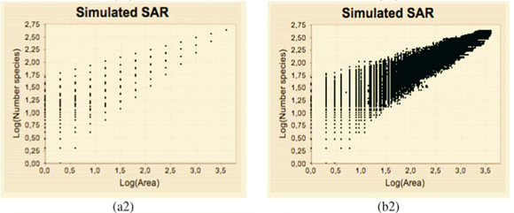
The plots of the simulated (S, A) data exhibit a dispersion of the values which increases when A decreases in a way which is qualitatively very similar to those of observed data (not shown). The estimation of (q) using the new algorithm includes all the scales where enough data are available (i.e. many dots are involved in the linear regression exhibited on Fig. 3(b)(3)).
Numerical experiments showed that adding a residual correction involving є(r) to complete the pseudopartition of the multifractal object was important to get reliable estimates. This type of correction should be applied also for the determination of the fractal dimension of irregular objects. When q = 0, the method of estimation of D(0) is identical to the box-counting method used to estimate a fractal dimension D and D(0) = D. In our example, the support of the richness measure is the entire planar Ω domain and one should have D(0) = D = 2 for this purely Euclidean support. We found that when the correction є(r) is omitted, the numerical estimates deviate significantly from the expected 2 value [Fig. 3(b3)] and that the results become correct when the correction is introduced [Fig. 3(b4)]. Tests were then carried out for a large range of q values on many virtual maps. An example is shown in Fig. 4(a3), where several values are plotted for a same given map. The variability of the numerical estimates is due to the random selection of (S, A) values, which occurs at the stage of random sampling in the virtual structure as well as at the stage of random selection of the right amount of data in the D(q) algorithm. The dispersion of (q) around the theoretical values of D(q) is smaller for larger values of kmax [Figs 4(b3) and 4(c3)].
We conclude that the estimation of the approximate Renyi dimensions (q) using the above algorithm can be used on real data sets providing with sufficiently representative (S, A) values, and that the quality of the numerical estimates will be improved if the data are selected over a rather large range of scale.
Conclusion
We have developed an extension of classical multifractal algorithms to the case of random sampling of the number of species S found in arbitrary spatial domains of area A. The new algorithm uses arbitrary shapes to pave with pseudopartitions the domain studied instead of classical regular grids. This method can be useful in many fields of application, especially when the support of the measure is irregularly shaped and when exhaustive data are not available on the whole sampled domain at every scale. One objective of this paper was first to show how the construction of virtual maps enables useful numerical analysis as regards the characterization of multifractal spatial structures. It is impossible to tune a new algorithm on real data, not only because of noise or poor data quality, but because of intrinsic reasons: we do not know a priori which theoretical values are expected and how to check the algorithm. The tests carried out on simulated data show that despite the simplicity of the construction process of the virtual maps, scaling properties appear to hold in any irregular subpart of the domain, even when arbitrary sampling blurs the hard regularity of the visual pattern. As regards the applications to species richness data, we are in the process of applying the new algorithm to real data, and the results are promising, but the discussion of their ecological significance lies beyond the scope of the present methodological paper.
In this article, we described how a multifractal model can capture key parameters of real multiscale heterogeneous distributions via the construction of synthetic maps, even if the construction of these maps by iterative bisections does not mimic the genesis of the real world. We showed that such virtual maps can be easily generated on computer by means of a multiplicative cascade in repeated bisections. Currently, we are conditioning virtual maps on real data, that is, we generate virtual richness maps using values of p1 and p2 estimated from real data sets, via the estimated Renyi dimensions (q).
More generally and from a methodological point of view, multifractal virtual maps can be useful in many fields to enable the modelling of heterogeneous spatial structures where similar patterns occur over a large range of scales. Whatever the type of application, the conceptual framework and associated simulations will be useful for research where paramaterizable models of spatial structures are required to investigate the implications of spatial variability for ecosystem dynamics.
1. Lovejoy S. and Shertzer D. (2006). Multifractals, cloud radiances and rain. J. Hydrol. 322, 59–88. [ Links ]
2. Lovejoy S. et al. (2001). Universal multifractals and ocean patchiness: phytoplankton, physical fields and coastal heterogeneity. J. Plankton Res. 23, 117–141. [ Links ]
3. Rodrigueziturbe I., Marani M., Rigon R. and Rinaldo A. (1994). Self-organized river basin landscapes: fractal and multifractal characteristics. Water Resources Research 30, 3531–3539. [ Links ]
4. Ozik J., Hunt B. and Ott E. (2005). Formation of multifractal population patterns from reproductive growth and local resettlement. Phys. Rev. E 72, 513– 519. [ Links ]
5. Harte D. (2002). Multifractals: Theory and Applications. Chapman and Hall, CRC, Boca Raton, FL. [ Links ]
6. Schmiegel J., Barndorff-Nielsen O. and Eggers H. (2005). A class of spatio-temporal and causal stochastic processes, with application to multiscaling and multifractality. S. Afr. J. Sci. 101, 513–519. [ Links ]
7. Perrier E., Tarquis A. and Dathe A. (2006). A program for fractal and multifractal analysis of two-dimensional binary images: computer algorithms versus mathematical theory. Geoderma 134, 284–294. [ Links ]
8. Perrier E., Mullon C., Rieu M. and de Marsily G. (1995). Computer construction of fractal soil structures: simulation of their hydraulic and shrinkage properties. Water Resources Research 31, 2927–2943. [ Links ]
9. Rosenzweig M. (1995). Species Diversity In Space and Time. Cambridge University Press, Cambridge. [ Links ]
10. Stanley H. and Meakin P. (1988). Multifractal phenomena in physics and chemistry. Nature 335, 405–409. [ Links ]
11. Harte H., Kinzig A. and Green J. (1999). Self-similarity in the distribution and abundance of species. Science 284, 334–336. [ Links ]
12. Perrier E. (2007). Online at: www.ird.fr/ur079/perso/perrier/MFspecies/Applet MFspecies.htm [ Links ]
* Author for correspondence. E-mail: henri.laurie@uct.ac.za

