BIOLOGICAL MODELLING

 

A time discrete linear model of an age and time of residence structured population in a patchy environment

 

 

A. Moussaoui^{I, II, *}; P. Auger^I; M. Khaladi^III; N. Ghouali^II

^IIRD UR GEODES Centre IRD de l'Île de France, 32 Avenue Henri Varagnat, 93143 Bondy Cedex, France
^IIDépartement de mathématiques, Faculté des Sciences, Université Aboubekr Belkaid-Tlemcen, Algeria
^IIIDépartement de Mathématiques, Faculté des Sciences Semlalia, Université Cadi Ayyad de Marrakech, Morocco

 

 

---

ABSTRACT

We present a multiregional Leslie matrix population model for an age-structured population in a heterogeneous environment of patches connected by migrations. The aim of the model is to take into account the time of residence of individuals in the patches. We present an application of the model in ecotoxicology. We consider a population located on two patches with a polluted patch whereas the other one is unpolluted. We study the effects of pollutant concentration and of the time of residence in the polluted patch on the global population growth rate. The model could be generalized to the case of N patches (N > 2) for Salmo trutta and cadmium concentration.

---

 

 

Introduction

Structured population models of discrete type have received varying degrees of attention. Ecologists, mathematicians and population biologists have observed that structure variables provide more realistic results than global models at reasonable computational expenses for a wide variety of biological populations. For example, biologists have observed that most exploited fish populations migrate or are confined to some preferential habitats at certain stages of their life cycle. Fishermen may follow some of these spatial and seasonal patterns, in which case the spatio-temporal distribution of fishing effort is closely tied to that of fish abundance.¹ We therefore need a state vector giving the number of individuals of different ages and at different locations. A list of ecological applications can be found in refs 2–4.

Most animal species exploit resources distributed in discrete patches in the environment, and natural selection should favour individuals that exploit such patchily distributed resources most efficiently. In this context, optimal foraging theory predicts that animals should optimize their patch residence time to maximize the rate at which resources are encountered and exploited.

To describe this behaviour, a Leslie matrix model is coupled to a dispersal matrix model, leading to a large class of models — the multi-regional Leslie models. Such models do not take into account the time spent by individuals in the different patches of the environment. In several cases, however, it is crucial to take into account the residence time that individuals spend in the different patches. For example, in ecotoxicology, the survival of an individual can depend upon the amount of pollutant accumulated in the organism. Survival does not therefore depend only on the actual presence of an individual in a polluted patch but rather on the total time it has already spent in this patch throughout its life. When individuals have spent several years at the same patch, they have gained experience which can be an advantage for survival and for reproduction with respect to individuals that settled on that patch only recently. The aim of this article is to take into account the time of residence in different patches in a multi-regional Leslie matrix model and to examine its effects on the global growth of a structured population living in a set of patches connected by migration and dispersal. We shall present an application in ecotoxicology by considering the case of a set of two patches, with one patch being polluted and the other not.

We classify individuals by the spatial patch they are in, their age and the time spent in the patch, and we take pollutant effects into account. The goal here is to estimate population responses to increasing pollutant concentrations. The outputs of our model are asymptotic population growth rate, stable age distribution for each age class, and asymptotic residence time, these variables being functions of the pollutant concentration.

The paper is organized as follows: In the following section, we present the general mathematical multi-regional Leslie model with time of residence. The next section is devoted to the study of an example in ecotoxicology. We consider a numerical example where we present the consequences of increased concentrations of toxicants in the natural environment on stable age structure, the asymptotic spatial distribution, the asymptotic population growth rate, and on the asymptotic residence time. We give sufficient conditions to exhibit strong ergodicity (tendency towards a fixed population structure independent of the initial conditions). This work has been inspired mainly by the paper by Arino and Smith.⁵ These authors presented a linear continuous model for age-structured populations which migrate between several locations, taking into consideration the time spent in a given area.

 

Notation, models, and basic results

Let us consider a population of N (>2) individuals divided between 2 patches (sites) and q age classes. We classify individuals by the spatial patch they are in, the age and the time spent in the patch, and we allow migration-survival and migration-fertility rates to depend on these three factors. The model includes two processes, demography taking into account the birth of each individual as well as the transition between different age groups, and migration characterizing the change of spatial patch. We assume that the length of time spent in each age class is the same as the projection interval. Parameters are assumed to be constant over time.

The following notation is used throughout:

An individual belongs to age class a at time t if its age is between a – 1 and a at time t.

For an individual in age class a, we denote by k the total cumulative residence time in patch i (i = 1, 2) from birth to age a (thus, the residence time in the second patch is a – k).

• Let (t)be the number of individuals in age class a living on patch i (i=1, 2) at time t which have accumulated a residence time k on patch i (i = 1, 2) and a – k on the second patch.
• Let be the newborn number in patch i per individual in age class a whowas in patch j one step of time ago, with time of residence k on patch j.
• Let be the proportion of survivors in patch i per individual in age class a whowas in patch j one step of time ago, with time of residence k on patch j.

The total population in patch i is given by:

The migration-survival model reads as follows:

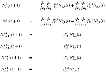
When k = 1…, a – 1, we obtain the next equations:

To simplify the presentation of the model, we introduce the following notations:

which is an a × 1 matrix (vector) of numbers of individuals aged a in patch i (i = 1, 2); with different residence time distributions, and where T denotes the transposition. We also define:

which is a 2a × 1 matrix (vector) of numbers of individuals aged a. The composition of the total population is then given by vector N(t) = (N¹(t), N²(t);…, N^q(t))^T.

is the 2 × 2a fecundity matrix per individual aged a (a > 1).

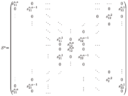
is the 2(a + 1) × 2a migration-survival matrix of individuals from age a to a + 1 (a > 1). In particular, S¹ is the migration-survival matrix from birth to age 1.

Therefore, if we consider a fixed projection interval, the rate of change for the whole population during that interval is then:

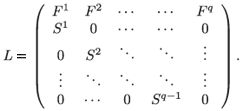
Finally, the global model describing the rate of change for the whole population N consists of the following system of q(q + 1) difference equations

N(t + 1) = LN(t),

where L generalizes the well-known Leslie (1945) matrix, with scalar fecundity and survival parameters replaced by 2 × 2a and 2(a + 1) × 2a matrices, respectively.

Mild conditions of connectivity between patches and age classes ensure that L is irreducible and primitive (ref. 3, p. 81; ref. 6, p. 30), according to the Perron-Frobenius theorem (ref. 3, p. 83; ref. 4, p. 4). L has a real positive dominant eigenvalue λ, which is simple. λ is the largest positive root of

det(L - λI) = 0.

The corresponding left and right eigenvectors v* and u* are positive and verify:

Lu* = λu*,

v*T L = λv*T

which are usually scaled such as v*^T u* = 1: Then:

N(t) = (v*^T N(0)) λ^tu*.

The multi-patch model thus obeys the well-known asymptotic exponential growth regime.^7,8 u* represents a stable age by patch structure; v* represents age by patch reproductive values.

 

Effects of pollutant on demography

In a previous contribution,⁹ we presented a mathematical model describing Salmo trutta (salmon) population dynamics in an arborescent river network. In this model, we coupled a Leslie matrix taking into account the ageing and reproduction processes to a migration matrix describing the fish patch changes in the river network. The river network was arborescent with four levels of arborescence, in which small rivers at any level were gathering to give birth to bigger rivers at the next level, and so on. This first contribution aimed at looking for the effects of river management such as building channels and dams on the global growth rate of the fish population. A further contribution¹⁰ aimed at taking into account annual spawning migrations in the model. The three next contributions focused on effects of pollutants on the fish population dynamics.^9–11 These papers again considered Salmo trutta and the effects of cadmium as pollutant on the global dynamics of the fish population. We focused on that species and that pollutant because data are available on the effects of chronic cadmium pollution on survival and fecundity of this fish. In these models, we considered that patch changes were rapid in comparison with reproduction and mortality, which allowed us to use aggregation methods in order to reduce the initial complete model into a global Leslie matrix model, governing the total number of fishes in the different age classes of the total network. It was thus possible to obtain a global response of pollution on the dynamics of Salmo trutta, given by the dominant eigenvalues of the aggregated model representing the global asymptotic growth rate of the population. We examined several scenarios according to different cadmium concentrations released at different levels of the network.

In these previous contributions, we had not taken into account the time of residence of the fish in the different patches. However, it appears acceptable to think that when a fish can move in a river network represented by a network of patches connected by migrations, such as in refs 9 and 10, the amount of pollutant ingested by a fish depends on the average time of residence it has spent in polluted patches, which in turn determines its ability to survive and reproduce. In this section, we shall consider the case of a general network of patches. The example presented here could apply to a Salmo trutta population and to chronic cadmium pollution

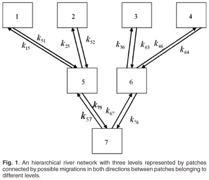
We will now examine a simple numerical example in ecotoxicology with only two patches. The model could be extended easily to N (N > 2) patches in a river network with hierarchical levels from upstream to downstream such as in refs 9–13. A possible example of river network with three levels is shown in Fig. 1. First we present the case of absence of toxicant. Second, we study the effect of pollution on the global asymptotic population growth rate, mean residence time, asymptotic residence time and on spatial distribution.

 

 

We consider a population structured in three age classes. Under these assumptions, there are twelve variables, ( i = 1, 2, a = 1, 2, 3, k = 1, 2, 3). We consider a particular example of a multi-regional Leslie matrix with time of residence written as follows:

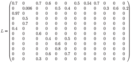
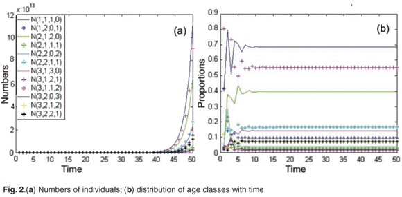
First, we simulated the population growth in the absence of toxicant. Figure 2(a) shows the time evolution of age and patch population numbers for the initial population vector X(0) = [100; 140; 150; 200; 120; 170; 160; 300; 400; 550; 820; 300]^T. The model was run for 50 months (month = 1 unit of time). In this example, the asymptotic population growth rate was equal to λ = 1.68. As shown in Fig. 2(b), the relative proportions of age class converge to a stable distribution.

 

 

Let us now consider a new case where a pollution discharge occurs in patch 1.

In that case, the matrix population model depends on pollutant concentration and can be written in general as follows:

where

and where Sª(C) is the proportion surviving from age a to age a + 1; and Fª(C) is the fecundity of individuals of age a at a given toxicant concentration C and where a = 1,…, q – 1.

Obviously, daily demographic rates must decrease as a function of toxicant concentration and of residence time in the polluted patch. Therefore, we use a decreasing logistical model as follows:

and

where , are the natural survival and fertility rates, respectively. Figure 3 shows the function α(C, s), which is a survival reduction function for a given toxicant concentration C corresponding to a population having a time of residence equal to s in patch 1, and γ and β are positive parameters.

 

 

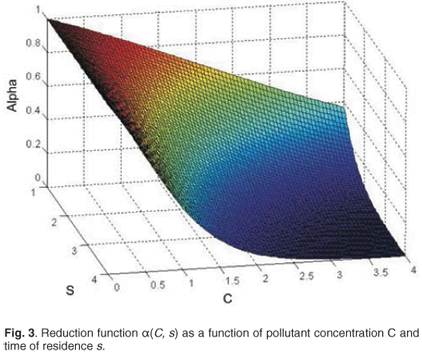
The logistical Equation (2) is a decreasing function of toxicant concentration C and of cumulative time of residence in patch 1.

The effects of toxicant on population dynamics will subsequently be quantified from the population growth rate λ, corresponding to the first eigenvalues of L(C).

The effect of pollution on population growth rate

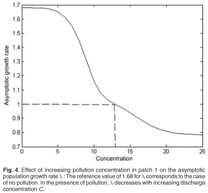
For C varying from 0 to 40, the decrease in λ as a function of toxicant concentration was simulated from population model (1). Toxicant had a major effect on asymptotic population growth rate λ, which rapidly decreased when the toxicant concentration increased. Above a concentration threshold of about 14, pollution leads to population extinction (λ < 1) (Fig. 4).

 

 

Effects of pollutant on residence time

The mean residence time in each patch for individuals aged a at time t is defined as follows:

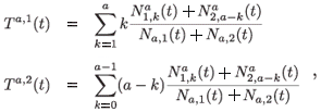
where N_a,i(t) is the total population aged a on patch i:

For any t, we have the next relation:

T^{a, 1} (t) + Tª^{, 2} (t) = a

Our general assumptions for this section are:

1) There is at least a non-zero coefficient in the last age class, that is, F^q ≠ 0. Moreover, there exists j such that g.c.d.(j, q) = 1 and there is at least a non-zero fertility coefficient in age class j(F^j ≠ 0).

2) For any age class, there is at least a non-zero survival coefficient, i.e. Sⁱ ≠ 0 for all i = 1,…, q.

The above assumptions guarantee that all results developed in this section are valid for our example of an age and patch-structured model (see refs 3, 4, 14, 15). Then, the system will asymptotically have a fixed growth rate and a fixed population structure, that are given by λ and V, respectively.

The asymptotic time of residence in patch 1 for individuals aged a is defined as follows:

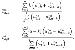
where

are the normalized (by total population) right eigenvectors for patch i, respectively, associated with the dominant eigenvalue of the multi-regional Leslie matrix with time of residence.

Let us define a global time of residence in patch 1 for the population as follows:

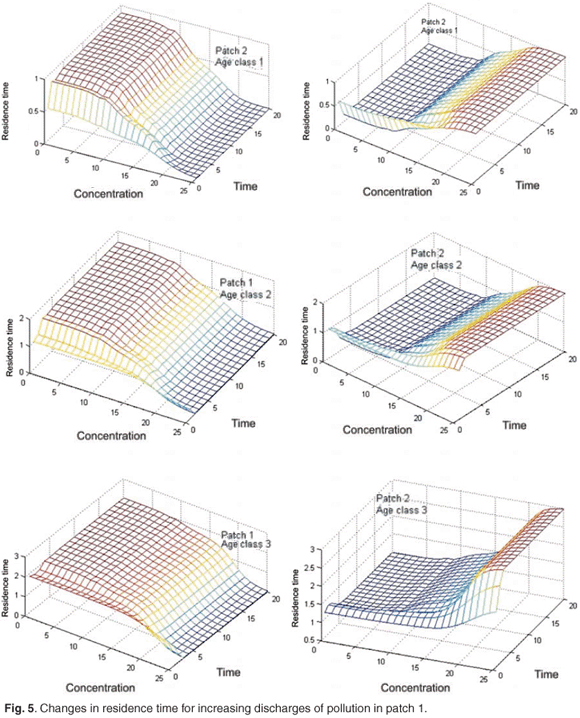
Figure 5 shows the changes in the mean residence time when the concentration of toxicant increases from 0 to 25 units in patch 1; we can see that the toxicant affects residence time.

 

 

Effects of pollutant on the global asymptotic residence time

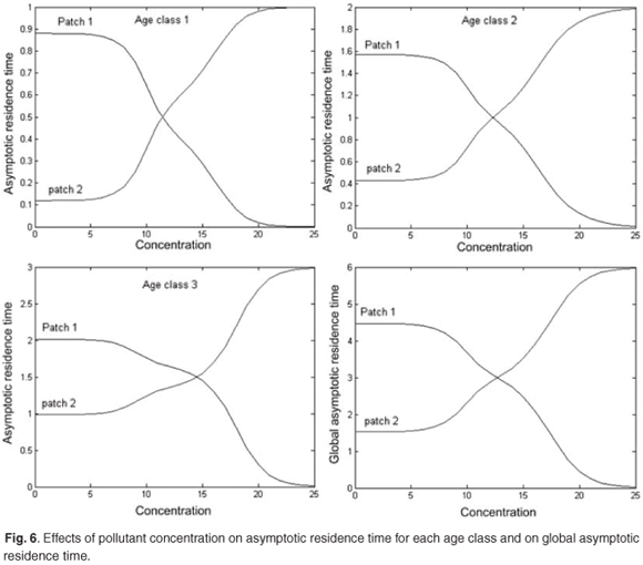
Figure 6 presents reduction in asymptotic residence time for each age class and on the asymptotic global residence time for increasing discharges of pollution in patch 1 when the concentration of toxicant increases from 0 to 25 in patch 1. Figure 6 shows that the toxicant has an important effect on residence time and on distribution of the population between patches.

 

 

Change in the spatial distribution

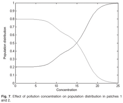
We now present the results for the spatial distribution when the discharged pollution concentrations are increased in patch 1. The distribution is symmetrical. Figure 7 shows that population switches from patch 1 to unpolluted patch 2.

 

 

Conclusion

Fish populations are examples of migratory effects playing an essential role. Most fishes are born in some place where adults meet during the reproductive season, and then mature elsewhere, the nurseries. Our study shows how a metapopulation with residence time could be used in an ecological framework in order to explore the effect of spatial distribution and contamination on population growth. Our multi-regional Leslie model presented in this paper could be used to describe the dynamics of a population travelling between two specific areas. It takes into consideration the time spent in a given area. Under some general conditions, it has been shown that the population verifies the ergodic property. This model is employed to assess the consequences of increased concentrations of toxicants in the natural environment on the population dynamics. We have demonstrated that the asymptotic population growth rate, the stable age structure, the asymptotic spatial distribution and the asymptotic residence time of a population living between two patches, vary in response to pollution concentration.

The model developed here can be extended to any number of patches. However, in most cases, we can consider a two-patch system only, with a zone 1 of patches where pollutant is present, and a zone 2 of patches with no pollution.

In future work, we wish to apply this general model with time of residence to several concrete examples such as the case of Salmo trutta and cadmium.^9,13 We believe that this general approach is pertinent to many real-life cases, and different species, different toxicants and different heterogeneous environments in terrestrial as well as aquatic environments.

 

1. Pelletier D. and Magal P. (1996). Dynamics of a migratory population under different fishing effort allocation schemes in time and space. Can. J. Aquat. Sci. 53, 1186–1199.        [ Links ]

2. Auger P. and Bravo De La Parra R. (2000). Methods of aggregation of variables in population dynamics. C.R. Acad. Sci. Paris Sci. de la vie, 323.        [ Links ]

3. Caswell H. (1989). Matrix Population Models. Sinauer Associates, Sunderland, MA.        [ Links ]

4. Cushing J.M. (1998). An introduction to structured population dynamics. CBMS- NSF, Regional Conference Series in Applied Mathematics, University of Arizona, Tucson, AZ.        [ Links ]

5. Arino O. and Smith W.V. (1998). Migration in age structured population. Math. Models Methods Appl. Sci. 8(5), 905–925.        [ Links ]

6. Berman A. and Plemmons R.J. (1994). Nonnegative Matrices in the Mathematical Sciences. Classics in Applied Mathematics. SIAM, Philadelphia.        [ Links ]

7. Lebreton J. and Gonzalez-Davila D.G. (1993). An introduction to models of subdivided populations. J. Biol. Syst. 1(4), 389–423.        [ Links ]

8. Lebreton J.D. (1996). Demographic models for subdivided populations: the renewal equation approach. Theor. Popul. Biol. 49, 291–313, 665–674.        [ Links ]

9. Charles S., Bravo De La Parra R., Mallet J.P., Persat H. and Auger P. (1998). A density dependent model describing Salmo trutta population dynamics in an arborescent river network: effects of dams and channelling. C. R. Sér. III, 321, 979–990.        [ Links ]

10. Charles S., Bravo De La Parra R., Mallet J.P., Persat H. and Auger P. (2000). Annual spawning migrations in modelling brown trout population dynamics inside an arborescent river network. Ecol. Model. 133(1–2),15–31.        [ Links ]

11. Chaumot A., Charles S., Flammarion P., Garric J. and Auger P. (2002). Using aggregation methods to assess toxicant effects on population dynamics in spatial systems. Ecol. Appl. 12(6), 1771–1784.        [ Links ]

12. Chaumot A., Charles S., Flammarion P. and Auger P. (2003). Ecotoxicology and spatial modelling in population dynamics: an illustration with brown trout. Environ. Toxicol. Chem. 22(5), 958–969.        [ Links ]

13. Chaumot A., Charles S., Flammarion P. and Auger P. (2003). Do migratory or demographic disruptions rule the population impact of pollution in spatial networks? Theor. Popul. Biol. 64, 473–480.        [ Links ]

14. Bravo de la Parra R. and Sanchez E. (1998). Aggregation methods in population dynamics discrete models. Math. Comp. Model. 27, 23–39.        [ Links ]

15. Sanz L. and Bravo De La Parra R. (1999). Variables aggregation in time discrete linear model. Math. Biosci. 157, 111–146.        [ Links ]

 

 

* Author for correspondence. E-mail: moussaouidz@yahoo.fr