BIOLOGICAL MODELLING

 

Chaotic linear systems in mathematical biology

 

 

J. Banasiak

School of Mathematical Sciences, University of KwaZulu-Natal, Durban 4041, South Africa; and Instytut Matematyki Politechnik Łódzkeij, ul. Wólczańska Łódź, Poland. E-mail: banasiak@ukzn.ac.za

 

 

---

ABSTRACT

Chaotic phenomena occurring in the natural sciences have been a focus of interest of both theoreticians and experimentalists for over five decades. Usually associated with nonlinear systems, they can also appear in infinite dimensional linear ones; that is, governed by, for instance, infinite systems of ordinary differential equations or partial differential equations. In this paper we shall provide a survey of mathematical tools which are necessary to analyse chaotic linear systems and discuss several examples of such systems arising in mathematical biosciences, ranging from drift-diffusion processes, through mutations, to the production of blood cells. We shall also attempt to address some questions related to the relevance of the mathematical analysis to properties of real-life systems.

---

 

 

1. Introduction

Chaotic behaviour typically is associated with nonlinear phenomena. The original example of chaotic evolution, given in the paper of Lorentz,¹ and all the subsequent results on chaotic behaviour of solutions to ordinary differential equations, refer to nonlinear systems; that is, in the equation

where '^•' denotes the time derivative, the function f is nonlinear (possibly acting in a multidimensional space ⁿ, in which case u = (u₁,..., u_n)). In the Lorentz example we had n = 3, f = (f₁, f₂, f₃) with f₁(u₁, u₂, u₃) = 10(u₂ - u₁), f₂(u₁, u₂, u₃) = -u₁ + 28u₁ - u₁u₃, f₃(u₁, u₂, u₃) =

In the last few decades, however, it has been observed that linear dynamical systems also can display a chaotic behaviour but for this they must be infinite dimensional. This means that the function f on the right-hand side of (1.1) must be, for instance, an infinite matrix, or a differentiation operator. That a finite dimensional linear system cannot produce chaotic behaviour should be intuitively clear: using the Jordan decomposition of a matrix we see that any finite dimensional linear dynamics is a superposition of finitely many simple ones (exponential, polynomial and trigonometric) and this cannot lead to any unexpected outcome.

First, we have to specify what is meant by a chaotic behaviour. There are several different, and not always equivalent, definitions of chaos; see ref. 2. The original idea, which appeared in Lorentz's paper,¹ was that the solutions to (1.1) for large times behaved in a strange and unpredictable way. This characterization is prevalent today within physics and applied mathematics, and in modern language it is phrased as the system having a strange attractor. We shall not develop this notion further as, from the mathematical point of view, this concept is very difficult to work with, see ref. 3, and also it is not relevant to linear systems. Also, we shall not dwell on another popular approach to chaos based on the measure theory and ergodic properties of the system (see e.g. refs 4-6). Instead, we shall focus on the so-called topological definition of chaos and from many (to a certain extent equivalent) definitions we have chosen the one introduced in ref. 7.

Before stating this definition, we must make sure that we know what we are talking about. We start with an explanation of the dynamical system. First, when we are talking about a system, we mean a variable describing the state of the system. The same real (physical, biological, etc.) system may then be represented in many ways. If we are interested in, say, the evolution of the average temperature of a body, then, at each time, the state of the system will be described by a single variable, and thus the system will be one-dimensional. If we want to know the temperature of each point of the body, then for each time the state of the system is described by a function of three spatial variables; in such a case the system is infinite-dimensional because the set of all, say, continuous functions is not a finite dimensional linear space.

Hence, we describe the system by a variable taken from some set which is called the state space. Although in principle the state space may be any set, in what follows we shall require that it is at least a topological space so that the concept of neighbourhood of a point can be properly defined. However, most consideration will be carried out in a much narrower class of Banach spaces (linear spaces with a translation invariant and homogeneous metric).

A dynamical system is one whose state x ∈ X (X is the state space) changes with some parameter t (time). Two main types of dynamical systems occur in applications: those for which the time variable is discrete (like the observation times) and those for which it is continuous. Our main interest lies with continuous dynamical systems. The dynamics is usually described by a differential equation

where the operator A, which describes mechanisms driving the system, is called its generator. Precisely speaking, by a continuous dynamical system we understand a family of functions (operators) (G(t))_t>0 such that for each t, G(t)x is a continuous function of x, for each x the function t → G(t)x is continuous with G(0)x = x, and for t > 0 and for x₀ from a sufficiently large subset of X [called the domain of the generator A and denoted by D(A)], the function x(t) = G(t)x₀ is a solution of the Cauchy problem

It is worth noting that if the solution to this problem is unique, then it has the following important property

which expresses the fact that the final state of the system can be obtained as the superposition of intermediate states. From the algebraic point of view, the above equation tells us that the dynamical system has a semigroup structure and therefore, especially in the linear case, it is called a semigroup of operators.

To define a chaotic dynamical system, we have to introduce the relevant terminology and notation. The orbit of (G(t))_t>0 originating from x ∈ X is the set {G(t)x}_{t> 0}. We say that (G(t))_{t> 0} is topologically transitive if for any two non-empty open sets U,V ⊂ X there is t₀ > 0 such that G(t₀)U ∩ V ≠ . Finally, a periodic point of (G(t))_{t> 0} is any point x ∈ X satisfying G(τ)x = x for some τ > 0.

Definition 1.1. Let X be a metric space.⁷ A dynamical system (G(t))_{t> 0} in X is said to be (topologically) chaotic in X if it is topologically transitive and its set of periodic points is dense in X.

Historically speaking, Devaney's definition of chaos contained one more condition: sensitive dependence on initial data (sdic), which commonly is regarded as a core property characterising chaos. However, it can be proved⁸ that topological transitivity and density of periodic points yield sdic.

Devaney's chaos is closely related to the property called hypercyclicity: a dynamical system (G(t))_{t> 0} is called hypercyclic if there is an orbit of (G(t))_{t> 0} which is dense in X; that is, it passes arbitrarily close to any point of X.

It turns out that hypercyclicity of a dynamical system is equivalent to its topological transitivity.⁹ Thus, Devaney's definition means that (G(t))_{t> 0} is chaotic if it has an orbit dense in X and its set of periodic points is dense.

 

2. Linear chaos

From now on we shall focus our attention on linear dynamical systems. A dynamical system (G(t))_{t> 0} is linear if for each t > 0 the operator G(t) is a linear bounded operator. In this case the generator A is also a linear, but not necessarily bounded, operator.

Even in this, in principle simpler, case proving chaoticity of a given dynamical system is not straightforward. Possibly the first systematic approach to determine whether a given linear system is chaotic was developed in ref. 10. It states (see Appendix A) that (G(t))_{t> 0} is chaotic if the point spectrum of its generator A contains an open set Ω in the complex plane , which intersects the imaginary line and, moreover, each set of eigenvectors corresponding to, respectively,

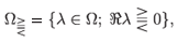
spans X. The last condition is usually quite difficult to check and that is why in Theorem A.2 we see a weaker requirement that there is a selection Ω ∋ λ → x_λ of eigenvectors which is an analytic function, and whose range spans X. Recently, in ref. 11, the authors observed that the existence of such an analytic selection of eigenvectors in Ω alone (that is, without the assumption that its range spans X) suffices for the eigenvectors corresponding to each set to span the same space, say X_ch, in which (G(t))_t>0 is chaotic.

To describe such a situation in a general case, we introduce the following definition. If there exists a closed subspace X_ch which is invariant under (G(t))_{t> 0}and such that for some x ∈ X_ch, then we say that (G(t))_{t> 0} is sub-hypercyclic. Furthermore, if (G(t))_{t> 0} is chaotic in X_ch, then we say that (G(t))_{t> 0} is sub-chaotic. The subspace X_ch is called, respectively, the hypercyclicity (chaoticity) subspace for (G(t))_{t> 0}. Recently,^11,12 it has been proven that for (G(t))_{t> 0} to be sub-hypercyclic (respectively sub-chaotic) it is enough that the set of eigenvalues of A contains a subset of the imaginary axis of non-zero measure over which the corresponding selection of eigenvectors is strongly measurable (respectively weakly continuous). Then (G(t))_{t> 0} is hypercyclic (respectively chaotic) in the closed span of the essential range of this selection.

It is worth noting that while sub-chaos (sub-hypercyclicity) is a weaker property than chaos (hypercyclicity), they still indicate the existence of trajectories oscillating between points of arbitrary small and arbitrary large magnitude (since X_ch is a nontrivial linear space). Thus, from the point of view of, say, numerical analysis, subchaos is as bad as chaos itself.

It is equally important to distinguish cases when the dynamical system cannot be chaotic, even in a subspace. To this end, we note that, by Theorem A.4, the only subspace in which the semigroup could be chaotic is the complement of the space spanned by all eigenvectors of the adjoint to the generator A. Hence, if this complement is finite dimensional, then the semigroup cannot be subchaotic as there are no chaotic linear systems acting in finite dimensional spaces. In particular, if the adjoint of the generator has an eigenvalue, then (G(t))_{t> 0} cannot be chaotic in the whole space X. Indeed, then the complement of the chaoticity space X_ch is nontrivial and thus X_ch ≠ X.

This result allows us to rule out important classes of semigroups from being hypercyclic. For example, the dynamical system generated by the diffusion equation on a bounded domain is not chaotic, as then the resolvent is a compact operator and the point spectrum of A* cannot be empty. However, if we remove the boundedness of the domain, the situation changes diametrically.

Example^10. On X = L₂([0, ∞)) we consider the equation

It follows that if a, b, c > 0 and c < b²/2a < 1, then the assumptions of Theorem A.1 are satisfied and the semigroup (G(t))_{t> 0} solving (2.5) is chaotic. Since the adjoint of the generator is given by 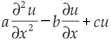with the same boundary condition, we obtain from Theorem A.4 that the dynamical system generated by

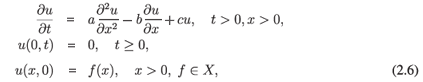
is not chaotic in any subspace of L₂([0, ∞)). These results can be intuitively explained by noting that the term in (2.5) describes flow towards the closed end x = 0 of the domain, whereas in (2.6) the term models flow towards the open end at x = ∞.

It is worth noting that there is a large gap between the sufficient and necessary criteria for chaos; at present any 'if and only if' result pertaining to the occurrence of chaos in general linear dynamical system seems to be far beyond our understanding of this phenomenon.

 

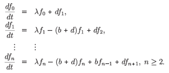
3. Birth-and-death type systems

Description of the models

Model 1. Development of drug resistance in cancer cells

A factor which can have a strong influence on the evolution of drug resistance of cancer cells is gene amplification. This process includes an increase in the number of genes responsible for coding a protein which aids either removal or metabolization of the drug. The more copies of the gene exist, the more resistant the cell, with the understanding that it can survive under higher concentrations of the drug. An increase in drug resistance by gene amplification has been observed in numerous experiments with in vivo and cultured cell populations. In addition, it has been established that tumour cells may increase the number of copies of an oncogene in response to an unfavourable environment. For further information, the reader is referred to refs 13-15, amongst others.

We consider a population of cancer cells stratified into subpopulations of cells of different types, labelled by numbers n = 0, 1, 2‚…. Because the biological process considered is gene amplification, cells of different types are identified as cells with different numbers of the drug resistance gene and therefore different levels of resistance. The cells belonging to 0-th subpopulation are sensitive to the drug. Due to a mutational event, the sensitive cell of type 0 can acquire a copy of the gene that makes it resistant to the agent. Likewise, the division of resistant cells can result in a change in the number of gene copies.

Empirical arguments support the hypothesis that the process described is subcritical; that is, in each cycle and at each level the probability of the decrease in the number of genes is greater than the probability of its increase. The randomness of the amplification process is modelled by a branching process.¹³ Since the number of gene copies can be very large, we use a model with an infinite number of cell subpopulations. As discussed in ref. 16, the infinite dimensional model provides a useful approximation of finite dimensional systems of arbitrarily high order, which are tractable only with numerical methods.

The process is characterized by two components: the conservative and the proliferative, which are described in detail below. The conservative component of the process describes the mutations of cells modelled as in a standard birth-and-death process. Here, α_nΔt, for n > 0, is the chance of one mutation in the n-subpopulation shifting the mutated cell to the n + 1-subpopulation, and δ_nΔt, for n ∈ , is the chance of one mutation in the n-subpopulation shifting the mutated cell to the n-1-subpopulation (we assume that d₀ = 0). The proliferative component is related to the assumption that the moment of death represents the moment of cell division with progeny of type n - 1, n or n + 1 and that the average life-span is given by the coefficient θ_n for the nth subpopulation (n > 0), described in detail below.

In practice, the same model arises in a context of microsatellite repeats.

Model 2. Microsatellite repeats

More than 95% of the human genome does not code any proteins. The non-coding DNA plays an organizational and regulatory role in the expression of genetic information. Large portions of non-coding DNA are organized in repeated sequences, which developed in different ways by amplification, transpositions or faults during replications. The shortest non-coding repeats of DNA are called microsatellites; they are repetitive sequences composed of 2-5 nucleotides and repeated 10-100 times. Formation of multiple repeats of such short units occurs most probably as a result of DNA replication errors in which slippage through the strand occurs. If not repaired, it gives rise to shortening or elongation of microsatellites with one or more repeated units. The stability of the number of repeats in a microsatellite sequence depends on the intact mismatch DNA repair and changes in the number of repeats accompany many diseases such as Huntington's disease, spinocerebellar ataxia type 1, the syndrome of fragile X chromosome or myotonic dystrophy; see e.g. refs 17-20. As mentioned above, the modelling is the same as in the case of gene amplificationdeamplification, only now the population is indexed by integers n = 0, 1,… corresponding to different variants of the number of repeats in the microsatellite. The interpretation of coefficients is similar.

To derive a mathematical model in both cases, following refs 13 and 20, we adopt the following assumptions:

• there exists denumerably many types of all particles, labelled with n = 0, 1,… ;

• the coefficients α_n and δ_n are probabilities of mutation (in a unit time) from n to n + 1 and n - 1 type, respectively;

• the life-spans of all particles are independent, identically distributed random variables with mean 1/θ_{n ;}

• upon its death, each particle of type n produces a pair of progeny, which survive independently with probability β_n and, for n > 1, independently of type n - 1, n + 1 or n with probabilities ν_n, η_n and 1 - η_n - ν_n, respectively;

• each progeny of an 0-type particle is of type 0.

Standard balancing argument produces the system

where we denote a0 = - λ₀ + b₀ and a_n = -λ_n + b_n + d_n for n ∈ .

The coefficients λ_n represent the proliferating term given by λ_n = θ_n(2β_n - 1), while b_n and d_n represent the conservative component and are given by

dn = 2βnνnθn + δn,

bn = 2βnηnθn + αn

To provide a rough idea of how the system (3.7) is derived, we note that the number of particles of type n increases due to the emergence of such particles at levels n - 1, and n + 1, represented here by the terms b_n-1f_n-1 and d_n+1f_n+1, respectively (note that the factor 2 corresponds to the fact that we are considering pairs of the progeny), and also by the production of type n progeny by type n parents, represented here by the term λ_nf_n. On the other hand, type n particles are lost in the same way, by giving birth to type n - 1, n and n + 1 particles, and by mutations. In the coefficients d_n and b_n, the first terms, respectively, correspond to creation of particles of new type by birth whereas the second terms represent mutations.

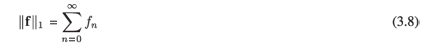
Stability results. We denote by f(t) = {f_n(t)}_{n> 0} the distribution function and by L the infinite matrix of the coefficients on the right-hand side of (3.7). The proper Banach space for the process defined by Equation (3.7) is the space l¹, where the norm

of any element f in the positive cone = {f ∈ l¹; f _n > 0, n= 0, 1, 2…} represents the total number of cells. For the sake of completeness, we shall consider also the Banach spaces l ^p < p < ∞, and c₀ (the space sequences converging to 0), with natural norms.

This model has been thoroughly investigated in the case of constant coefficients when the solutions can be found by Laplace transforms.^13,16,18,20 In the case of no mutations, the assumption that progeny of type-0 particles are themselves of type zero decouples the first equation from the rest (in the sense that the system for n > 1 can be solved independently of the first equation):

The interest in the papers cited above was in the asymptotic behaviour of the resistant cells' population, n > 1. Assume that f_n(0) = δ_1n and define

It was found that

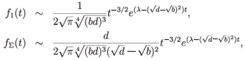
for t → ∞. Similar calculations can be done for other k. Thus, these solutions are exponentially stable provided

in addition to the subcriticality assumption d > b. Clearly, if this assumption is not satisfied, the functions f₁ and f_Σ grow exponentially fast with t → ∞. To the author's knowledge, the question whether constant coefficient birth-and-death type models can be chaotic in l ^p is still open. However, as described in Theorem 3.2, subchaos can be proved for a more general system with affine coefficient.

Variable coefficients - emergence of chaos. Constant coefficients are not always realistic. In ref. 22 the Equation (3.7) was considered under the assumption that the coefficients a_n, b_n (for n ∈ ₀), d_n (for n ∈ ) are nonnegative and

(A1) for some a > 0, a_n = a + α_n, n ∈ ₀, with α_n = 0,

(A2) for some d > 0 d_n = d,

(A3) lim b_n = 0.

To make these assumptions clearer, we note that the death-only systems with constant coefficients (b_n = 0, d_n = d and a_n = a with d > a) has been known to be chaotic for some time, see e.g. ref. 23. The results below can be interpreted as showing that the property of being chaotic persists when we consider small perturbations of such death systems with constant coefficients (including addition of a very small birth term). The exact form of the assumptions (A1)-(A3), and the constant q below, are related to the techniques of the proof.

Let _p, p ∈ [1, ∞[∪{0} denote the operator, defined by the matrix L of coefficients of (3.7), in l ^p and c₀, respectively. The operators _p are bounded, hence they generate dynamical systems (G_p(t))_t>0 in l^p and c₀, respectively.

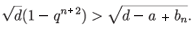
Theorem 3.1²¹. Let the ass umptions (A1), (A2) and (A3) be satisfied. There is q > 0 such that if |α_n|< dqⁿ⁺¹, |b _nd_n-1|< d²q²ⁿ⁺⁴ and a < d, then the semigroup generated by _p is chaotic in any l^p, 1 < p < ∞, and in c_0.

Consider the system transposed to (3.7)

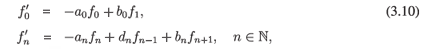
and, by Theorem A.4, if (3.10) was chaotic in any subspace, then the co-dimension of the span of all eigenvectors of the operator in (3.7) in respective space would be finite. Since this is not true, we have

Corollary 3.1. Suppose that the sequences (a_n), (b_n) and (d_n) are as in Theorem 3.1.²¹ Then the semigroup generated by (3.10) is chaotic in no subspace of l ^p, 1 < p < ∞, or of c₀.

Theorem 3.1 ensures the existence topological chaos for large deamplification ('death') rates and small amplification ('birth') rates, i.e. for the process which is subcritical. On the contrary, chaos will not appear in processes with small deamplification rates and possibly large amplification rates.

Let us compare our result with the stability result for the constant coefficients model. For simplicity, let d_n = d, a_n = a, a < d and satisfy |b_n|< dq²ⁿ⁺⁴; then λ_n = d - a + b_n and the stability condition (3.9) for our model reads

This condition clearly is satisfied for large n provided assumptions (A1)-(A3) hold. This apparent contradiction can be explained by noting that the asymptotic stability result (3.9) was obtained for positive data of finite length. Even more, results contained in ref. 18 show that no chaotic behaviour is possible if the initial distribution converges to zero sufficiently fast as n → ∞. On the other hand, chaos in this model is (probably) related to the possibility of infinitely many switches between negative and positive entries in initial conditions. Though this may seem to limit relevance of the above results for real life biological systems, Proposition 3.1 offers another way of interpreting them.

The assumptions of Theorem 3.1 are often too restrictive - in most standard applications the coefficients may grow with n. This creates numerous problems starting from the generation of the semigroup through the construction of eigenvectors to their density in l^p. In our analysis we adopt the following assumption.

Assumption AC. There exists N₀ > 1 with

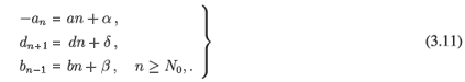
with a = -(b + d), b, d > 0, a, b, d ∈ .

Under these conditions one can prove^31,32 that the maximal operator associated with the infinite matrix on the-right hand side of (3.7), denoted _max, generates a semigroup. Then we have

Theorem 3.2²⁴. Suppose that 1 < p < ∞ and that Assumption AC holds with d > b and α + β + δ - (d - b)/p > 0. Then the semigroup generated by _max in l ^p is sub-chaotic.

Also in this case it is easy to see that the stability condition (3.9) is satisfied:

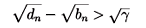
for large n provided b > d and yet the semigroup displays chaotic behaviour (though possibly in a subspace). We also have the following result, which rules out chaotic behaviour.

Theorem 3.3. Suppose that Assumption AC is satisfied, p ∈ [1; + ∞), and either (i) b > d, or (ii) d_m0 = 0 for some m₀ > 1. Then the semigroup generated by _max is not topologically chaotic.

It is worth commenting on the 'fragility' of the class of chaotic dynamical systems: according to (ii) it is enough to remove one entry of the infinite matrix L to switch from a chaotic to a non-chaotic system. The reason for this is that putting d_m0 = 0 decouples the system into a finite dimensional part, which is not chaotic, while the remaining infinite dimensional part may be chaotic at most in the proper subspace of l^p consisting of sequences having first m₀ entries equal to zero. On the other hand, if the system generated by _max is subchaotic, then putting d_m0 = 0 for some m₀ > 1 will not change this property. At present we do not know whether such a result is true in general; that is, whether subchaoticity of a system is preserved under finite-dimensional perturbations.

Interpretation of chaos. Let us reflect on the relevance of chaos for this particular model. In most biological applications only nonnegative solutions make sense and it is only fair to note that chaotic phenomena discussed here cannot occur for such solutions. In fact, for systems with strictly positive proliferation, the l₁ norm of any positive solution to (3.7) may only grow and hence the solution cannot wander.

On the other hand, as we are dealing with linear systems we may wish to consider the differences between two physical (i.e. non-negative) solutions and such a difference certainly need not be non-negative and it may be chaotic. In fact, we have

Proposition 3.1. If (G(t))_t>0 is a subchaotic semigroup, then for any є > 0 there exist x₁, x₂ > 0 such that ║x₁ - x₂║ < є and {G(t)x₁) - G(t)x₂)_t>0 is dense in the space of chaoticity of (G(t))_t>0.

In other words, the difference between two positive solutions which were arbitrarily close to each other at t = 0 may evolve in a chaotic manner.

Another way of looking at this question is discussed in the following example.

Example 3.1. Finite dimensional manifestation of chaos. Consider a pure death system with proliferation:

By Theorem 3.1 this system is always chaotic provided d > a. We can write down an explicit solution to this system

The eigenvector corresponding to eigenvalue λ is given by e_λ = (µ, µ²,..., µⁿ,...) where µ = ((λ + a)/d)ⁿ, provided |µ|<1.

Let us put a = 0.1, d = 10 and take the initial condition f₀ = ℜe_i = ℜ(i, i²,…, iⁿ,…), where i is the imaginary unit and ℜ denotes the real part of a complex number. As this corresponds to a purely imaginary eigenvalue, the solution of the full system is periodic.

For calculations, we took 100 × 100 cut-off of the solution (3.12) corresponding to the above eigenvalue and plotted the behaviour of two first coordinates for t = 10, 20, 30, 40.

 

 

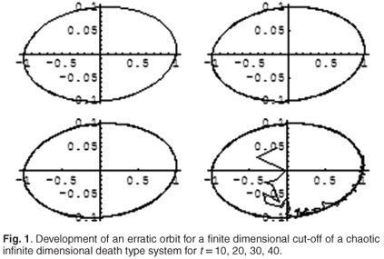
We see that a perfectly periodic orbit suddenly changes its behaviour. While this is not a proof that the dynamical system described by (3.12) is chaotic (after all, a 100 ×100 cut-off of (3.12) can be extended to an infinite system in many ways, including non-chaotic ones), it could, however, be an indication that the system has a potential to develop irregular behaviour.

 

4. Population models for the evolution of blood cells

Regular growth. Following ref. 25, we consider a population of blood cells distinguished only by their size and describe the population by the density function n(t, s) of cells having size s in time t. The following processes take place when the time passes:

1) Each cell grows in time with velocity g(s) depending on cell size s;

2) each cell dies with a probability µ depending on size;

3) each cell divides into two daughter cells of equal size with a probability depending on size.

Moreover, we assume that there exists a maximal cell size (here normalized to 1); also there exists a minimal cell size s = α > 0 below which no division can occur. As a consequence of the last assumption, if we start with an initial population with sizes greater that α/2, the size of each cell in the population must satisfy s > α/2 and we can assume the boundary condition u(t, α/2) = 0.

These assumptions lead to the following evolution equation:

where χ_A is the characteristic function of the set A. We assume that the death rate µ is a positive continuous function on [α/2, 1]. The division rate should be continuous with b(s) > 0 on (α, 1) and b(s) = 0 elsewhere. Moreover, g(s) is differentiable and satisfies 0 < є < g(s) < δ on [α/2, 1] and 2g(s) > g(2s) for s ∈ [α/2, 1/2].

We consider this equation as an evolution equation in X = L₁([α/2, 1], ds). One can prove that (4.13) generates a semigroup (G(t))_t>0 which is uniformly continuous, compact for t > 1 - α/2, and is also irreducible. Thus, (4.13) is a model example of the so-called asynchronous exponential growth, a property well known in population theory. This property can be expressed as

for any initial condition u₀, where n is the eigenvector corresponding to the dominant eigenvalue λ_max; n is called the stable size distribution. In other words, irrespective of the initial condition, after a short time the distribution of cells starts evolving as a scalar multiple of a fixed vector. Hence, the evolution definitely does not display any features of a chaotic behaviour.

Abnormal cell growth. In ref. 26 the author considered the growth rate g to be g(s) = s and deviated from the set of usual assumptions by assuming that:

4. there is an immigration of new cells from a regulatory source, allowing for renewal of the cell population at a rate ν(s) depending upon cell size;

5. cells of any size may divide.

The first assumption is not difficult to accept - in many biologically significant systems within an organism, such as in the production of blood, we recognize the need for a source. Since all cellular lines are dead ends, a source such as the precursor stem cells is needed to sustain a viable population. The second assumption amounts to setting α = 0 in (4.13) and allowing cells of any size to exist. While biologically the idea of having a cell of size 0 is unrealistic, this size is taken as a limiting value to describe an abnormality in the division process, resulting in the accumulation of cells in a population of non-functional 'dwarf' cells. The presence of such dwarf cells is seen in the blood disorder alpha-thalassemia, a genetic disease associated with sickle cell anaemia. This has the effect of greatly reducing the mean corpuscle volume of red blood cells.

We begin analysis of this model by first considering a simplified equation

Though the semigroup is given explicitly by

u(t, s) = [G(t)u₀] (s) = e^t/2u₀ (se^-t)

it is chaotic in the space C₀([0, 1]) (of continuous functions vanishing at 0) and in the spaces L_p([0, 1]), p > 1, see refs 5, 21, 27, 28. Interestingly enough, (4.14) does not generate a chaotic semigroup in the space of all continuous functions C([0, 1]). The fact that the semigroup is chaotic in C₀([0, 1]) but not in C([0, 1]) was attributed by Glenn Webb in ref. 28, p. 48 to the insufficient supply of the most primitive blood cells (with size 0) in the former case.

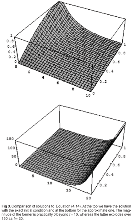
In this case, chaotic solutions are non-negative and thus are biologically relevant. We illustrate sensitive dependence of solutions on initial conditions by presenting exact solutions for the initial condition u₀(s) = sin s, s ∈ [0, 1] and for its approximation by the Fourier series of cosines truncated after 100 terms. The comparison of these two initial conditions is given in Fig. 2.

 

 

The comparison of solutions is given in Fig. 3. We see that the solution corresponding to the exact initial condition almost immediately decays to zero, whereas the one for the approximate condition reaches the level of over 150 in just 20 time units. This can be explained by noting that, due to the concentration of characteristics of (4.14) close to s = 0, the minute difference between the exact and approximated initial condition close to the origin will be exponentially magnified as time increases.

 

 

Consider next a variant of (4.13) modified so that the additional assumptions 4 and 5 are satisfied:

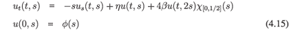
in X = L₁([0, 1], ds). The eigenvectors²⁹ are given by

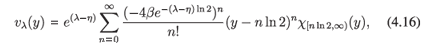
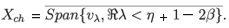
where y = -ln s, and they are analytic for ℜλ< η + 1 - 2β. Thus, if η + 1 - 2β > 0, then the assumptions of Theorem A.2 are satisfied and hence the dynamics generated by (4.15) is subchaotic in

Furthermore, using quite sophisticated results from complex analysis, the authors of ref. 29 showed that

X_ch = X;

that is, the dynamics is chaotic in the whole space, provided β < 1/2 ln 2.

 

1. Lorenz E.N. (1963). Deterministic nonperiodic flow. J. Atmos. Sci. 20, 130-141.        [ Links ]

2. Hill D.A. (2000). Chaotic chaos. Math. Intelligencer 22(3), 5.        [ Links ]

3. Viana M. (2000). What's new on Lorenz strange attractors? Math. Intelligencer 22(3), 6-19.        [ Links ]

4. Eckmann J-P. and Ruelle D. (1985). Ergodic theory of chaos and strange attractors. Rev. Mod. Phys. 57, No. 3, Part I, 617-656.        [ Links ]

5. Lasota A. and Mackey M.C. (1995). Chaos, Fractals and Noise, Stochastic Aspects of Dynamics. Springer-Verlag, New York.        [ Links ]

6. Rudnicki R. (2004). Chaos for some infinite-dimensional dynamical systems. Math. Meth. Appl. Sci. 27(6), 723-736.        [ Links ]

7. Devaney R.L. (1989). An Introduction to Chaotic Dynamical Systems, 2nd edn. Addison Wesley, New York.        [ Links ]

8. Banks J., Brooks J., Cairns G., Davis G. and Stacey P. (1992). On Devaney's definition of chaos. Amer. Math. Monthly 99, 332-334.        [ Links ]

9. Godefroy G. and Shapiro J.H. (1991). Operators with dense, invariant, cyclic manifolds. J. Funct. Anal. 98, 229-269.        [ Links ]

10. Desch W., Schappacher W. and Webb G.F. (1997). Hypercyclic and chaotic semigroups of linear operators. Ergodic Theory Dynam. Syst. 17, 793-819.        [ Links ]

11. Banasiak J. and Moszyński M. (2008). Hypercyclicity and chaoticity spaces of C₀-semigroups. Discr. Cont. Dyn. Sys. A 20(3), 577-587.        [ Links ]

12. El Mourchid S. (2006). The imaginary point spectrum and hypercyclicity. Semigroup Forum 73(2), 313-316.        [ Links ]

13. Kimmel M. and Stivers D.N. (1994). Time-continuous branching walk models of unstable gene amplification. Bull. Mah. Biol. 50, 337-357.        [ Links ]

14. Stark G.R. (1993). Regulation and mechanisms of mammalian gene amplification. Adv. Cancer Res. 62, 87-113.        [ Links ]

15. Windle B. and Wahl G.M. (1992). Molecular dissection of mammalian gene amplification: New mechanistic insights revealed by analysis of very early events. Mutat. Res. 270, 199-224.        [ Links ]

16. Kimmel M., Świerniak A. and Polański A. (1998). Infinite-dimensional model of evolution of drug resistance of cancer cells. J. Math. Syst. Estim. Control 8(1), 1-16.        [ Links ]

17. Bobrowski A. and Kimmel M. (1999). Dynamics of the life history of a DNA-repeat sequence. Arch. Control Sci. 9(45), No. 1-2, 57-67.        [ Links ]

18. Bobrowski A. and Kimmel M. (1999). Asymptotic behaviour of an operator exponential related to branching random walk models of DNA repeats. J. Biol. Syst. 7(1), 33-43.        [ Links ]

19. Kruglyak S., Durret R.T., Schug M.D. and Aquadro Ch.F. (1998). Equilibrium distributions of microsatellite repeat length resulting from a balance between slippage events and point mutations. Proc. Natl Acad. Sci. USA 95, 10774-10778.        [ Links ]

20. Świerniak A., Rzeszowska-Wolny J., Kimmel M. and Polański A. (1999). Asymptotic properties of microsatellite repeats model. In Proc. National Conference on Applications of Mathematics in Biology, Ustrzyki Gorne, 14-17 September, pp. 143-148.        [ Links ]

21. Banasiak J. and Lachowicz M. (2001). Chaotic linear dynamical systems with applications. In Semigroups of Operators: Theory and applications (Rio de Janeiro), pp. 32-44. Optimization Software, New York.        [ Links ]

22. Banasiak J. and Lachowicz M. (2002). Topological chaos for birth-and-death-type models with proliferation. Math. Models Methods Appl. Sci. 12(6), 755-775.        [ Links ]

23. Protopopescu V. and Azmy Y.Y. (1992). Topological chaos for a class of linear models. Math. Models Methods Appl. Sci. 2(1), 79-90.        [ Links ]

24. Banasiak J. , Lachowicz M. and Moszynski M. (2007). Chaotic behavior of semigroups related to the process of gene amplification-deamplification with cells' proliferation. Math. Biosci. 206(2), 200-215.        [ Links ]

25. Engel K-J. and Nagel R. (1999). One-Parameter Semigroups for Linear Evolution Equations. Springer-Verlag, New York.        [ Links ]

26. Howard K.E. (2001). A size structured model of cell dwarfism. Discrete Contin. Dyn. Syst. Ser. B 1(4), 471-484.        [ Links ]

27. Rudnicki R. (1988). Strong ergodic properties of a first-order partial differential equation. J. Math. Anal. Appl. 133(1), 14-26.        [ Links ]

28. Webb G.F. (1995). Periodic and chaotic behavior in structured models of cell population dynamics. In Recent Developments in Evolution Equations, eds A.C. McBride and G.F. Roach, Pitman Research Notes in Mathematics 134, 40-49. Longman Scientific & Technical, Harlow,        [ Links ]

29. El Mourchid S., Metafune G., Rhandi A. and Voigt J. (2008). On the chaotic behaviour of size structured cell populations. J. Math. Anal. Appl. 339, 918-924.        [ Links ]

30. Banasiak and Moszynski M. (2005). A generalization of Desch Schappacher Webb criteria for chaos. Discr. Cont. Dyn. Sys. A 12(5), 959-972.        [ Links ]

31. Banasiak J. and Arlotti L. (2006). Perturbations of Positive Semigroups with Applications. Springer, London.        [ Links ]

32. Banasiak J. (2004). A complete description of dynamics generated by birth-and-death problems: A semigroup approach. In Mathematical Modelling of Population Dynamics, ed. R. Rudnicki. Banach Center Publications, vol. 63, 165-176.        [ Links ]

 

 

Appendix: Criteria for existence of chaos

Sufficient criteria for chaos

Theorem A.1.¹⁰ Let X be a separable Banach space and let A be the generator of a semi-group (G(t))_t>0 on X. Suppose that

1) the point spectrum of A, σ_p(A), contains an open connected set U such that Uiℜ ≠ ;

2) There exists a selection U ∋λ → x_λ of eigenvectors of A that is analytic in U;

3)

Then (G(t))_t>0 is chaotic.

In many cases property 3 is the most difficult to establish. However, the following result paves a way to circumvent the problem.

Theorem A.2.³⁰ Suppose that conditions 1 and 2 of Theorem A.1 are satisfied. Then there exists an infinite-dimensional closed subspace Y (⊆) X, which is invariant under (G(t))_t>0, such that (G|_Y (t))_t>0 is chaotic.

This proposition justifies the definitions of sub-hypercyclic and subchaotic semigroups given in the main text. Another far-reaching generalization of Theorem A.1 is given below.

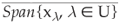
Theorem A.3.^11,12 Let A be the generator of a strongly continuous semigroup (G(t))_t>0 on a separable Banach space X. Assume that there is Ω := (ω₁, ω₂) ⊂ with µ(Ω) > 0 and a strongly measurable f : Ω → X such that Af (λ)= iλx(λ) for almost any λ ∈ Ω. Then ((G(t))_t>0 is sub-hypercyclic in X with a hypercyclicity space

Here, for a function f defined on a measure space (Ω, µ) with values in a Banach space X, f(Ω)_ess is the essential range of f; that is,

f(Ω)_ess = {x є X; µ({s є Ω :║f (s) - x║ < є}) ≠ 0, ∀є > 0},

Corollary A.1 If there is an interval I ⊂ Ω such that f(I) ⊂ f(Ω)_ess, then (G(t))_t>0 is sub-chaotic (with chaoticity space possibly smaller that X_ch).

Corollary A.2 Under notation of Theorem A.3, if Ω = [a, b] and λ → f(λ) is weakly continuous on Ω, then (G(t))_t>0 is chaotic in X_ch =

It is often suggested that a system with a sufficiently large number of periodic solutions should be chaotic. For linear systems, periodic solutions are solutions corresponding to imaginary eigenvalues, thus Theorem A.3 seems to be a step in right direction. However, one can construct a subspace of the space X = C_b() of bounded continuous functions on which the semigroup of translations

(G(t) f) (x) = f (t + x)

is a strongly continuous semigroup of isometries (and thus cannot be chaotic), while each point of the imaginary axis is an eigenvalue of its generator.¹¹

Necessary criteria for chaos. For a set M ⊂ X define the 'orthogonal' complement of M in the adjoint space X* as

M^⊥ = {f є X*; < f, x > = 0, ∀x є M}.

Then we have

Theorem A.4. Let (G(t)) _t>0 be a continuous linear dynamical generated by A in a Banach space X, having an orbit dense in some subspace X_ch ⊂ X. Then the adjoint A* of A and the dual dynamical system ((G*(t))_t>0 have the following properties:

(i) Let 0 ≠ ø ∈ X*. If the orbit {G*(t)ø} _t>0is bounded, then

(ii) If ø is an eigenvector of A*, then f ∈

In particular, if

σ_p (A*) ≠

then (G(t))_t>0 cannot be chaotic. Indeed, in this case is nontrivial and thus X_ch ≠ X. Furthermore, if the codimension of the linear span of all eigenvectors corresponding to σ_p(A*) is finite, then there is no subspace of X in which (G(t))_{t> 0} is chaotic.