


Servicios Personalizados
Articulo
 Inglés (pdf)
 Articulo en XML
 Referencias del artículo
Indicadores

Links relacionados
-
 Citado por Google
 -
 Similares en Google
Compartir

 Permalink
South African Journal of Science
versión On-line ISSN 1996-7489
versión impresa ISSN 0038-2353
S. Afr. j. sci. vol.104 no.3-4 Pretoria mar./abr. 2008
RESEARCH ARTICLES
Simulating atmospheric turbulence using a phase-only spatial light modulator
Liesl BurgerI, II; Igor A. LitvinI, III; Andrew ForbesI, II, *
ICSIR National Laser Centre, P.O. Box 395, Pretoria 0001, South Africa
IISchool of Physics, University of Kwazulu-Natal, Private Bag X54001, Durban 4000, South Africa
IIILaser Research Institute, University of Stellenbosch, Private Bag X1, Matieland 7602, South Africa
ABSTRACT
Demonstration of the effect of atmospheric turbulence on the propagation of laser beams is traditionally a difficult task. This is due to the complexities of long-distance measurements and the scarcity of suitable laser wavelengths in atmospheric transmission windows. We demonstrate the simulation of atmospheric turbulence in the laboratory using a phase-only spatial light modulator. We illustrate the advantages of this approach, as well as some of the limitations, when using spatial light modulators for this application. We show experimental results demonstrating these limitations, and discuss the impact they have on the simulation of various turbulence strengths.
Introduction
As a laser beam propagates through the atmosphere, it spreads laterally due to diffraction. This is a linear and deterministic property of all light propagation. It is often observed, however, that laser beams propagating through the atmosphere have a tendency to wander randomly about their propagation direction (rectilinear path), and appear to accumulate fluctuations in their light intensity, called scintillation (see Fig. 1). These two artifacts are also observed with the naked eye in the case of starlight: the so-called twinkling of the stars is precisely this randomness in path and intensity. It is now well understood that the origin of the randomness is atmospheric turbulence.1,2

While atmospheric turbulence is a stochastic process, there is 'structure' to the randomness. From an optical perspective, the theory of turbulent air is based on considering differences in refractive index between points in the atmosphere. Consider the Gladstone-Dale law that relates the density of air to its refractive index: the greater the density, the higher the refractive index. If random mixing of air of various densities takes place, the atmosphere will also appear random in refractive index. This mixing of the air is often driven by convective currents that move air packets of varying size around. The smallest eddies define the so-called 'inner scale', below which viscous effects are important, while the largest eddies define the so-called 'outer scale', above which the atmosphere can no longer be considered isotropic. Kolmogorov considered the simplified problem of a non-viscous and isotropic atmosphere, so that the inner scale is zero and the outer scale is infinity. These assumptions lead to a well-defined distribution for the randomness in the refractive index of the atmosphere, which can be applied in the laboratory, giving a good approximation for a real atmosphere.1,2 One of the key findings of Kolmogorov has been that the turbulence strength can be described by a single parameter, the atmospheric structure constant,  . If is large, the turbulence is strong, and vice versa. Typical values for range from 10–15 m–2/3 (high turbulence conditions near the ground) to 10–18 m–2/3 (low turbulence conditions at high altitude).
Not surprisingly, for applications where light must travel through the atmosphere, there are many active techniques to compensate for the effect of turbulence, for better 'vision' in astronomy, to superior signal delivery in telecommunications. The use of adaptive optics for atmospheric turbulence correction is fairly commonplace these days in both astronomical and military applications (see refs 1 and 2 for a good overview of the field). A modern optical element in the form of a spatial light modulator (SLM) has allowed new approaches to adaptive optics, and has already been recommended and used for the production of Zernike modes, adaptive optics and turbulence generation.3–7 Most of the approaches attempting to demonstrate turbulence have concentrated on Kolmogorov turbulence, and have made use of the SLM as the turbulence screen. Studies have concentrated on the impact of the turbulence on the laser beam and the use of SLMs as closed-loop correctors of turbulence.
We introduce the concepts of turbulence in this paper, and the use of spatial light modulators to describe turbulence. There are two basic aims: first, to expound on the steps required to actually simulate atmospheric turbulence in the laboratory, and second, to point out some of the limitations in using spatial light modulators as turbulence simulators, from a laser beam shaping perspective. That is to say, we are not so concerned with turbulence itself, but the impact of the SLM in simulating this turbulence. We will consider Kolmogorov turbulence as an example, and describe the effects of a single phase screen on the far-field intensity pattern of a laser beam. In the next section we will review the theory needed to create simple turbulence phase screens, and then show how to implement these in a laboratory situation. Finally, we highlight some limitations of using a spatial light modulator for this application.
Creating Kolmogorov phase screens
There are a few simple steps required to calculate a phase screen that represents turbulence. First, one must select an atmospheric turbulence model to use. Once done, the requirement remains that the selected turbulence model should somehow relate to the method used to describe the phase. The Zernike polynomials form a neat basis-set for representing optical phase with the convenient properties that: (a) the polynomial coefficients can be directly related to the known optical aberrations, (b) the polynomials are complete and orthogonal, and (c) the polynomial coefficients required to describe Kolmogorov turbulence can be calculated analytically. An introduction to Zernike polynomials is given in Appendix A.
The key equation is Equation (A7), which we repeat here for convenience:

In this context, Equation (1) implies that any radial phase function ø(ρ, θ) can be described as a sum of Zernike polynomials with weighting coefficients Anm and Bnm. The function ø(ρ, θ) may describe either surfaces of constant phase across an optical wavefront or a phase-only screen used to modify the optical wavefront. We will take the latter view in what is to follow, and use ø(ρ, θ) to describe the phase changes on the optical wavefront due to a turbulent atmosphere using the Kolmogorov theory of turbulence. Since in Kolmogorov turbulence Anm = Bnm, we will usually only refer to the Anm terms, which are sometimes called the even terms. In the case of creating a phase function that describes Kolmogorov turbulence, we use the Noll matrix approach,8 to find suitable values for A nm, after which the problem can then be solved.
Noll matrix
Kolmogorov turbulence screens can be created by calculating the spatial covariance matrix from the Zernike expansion of the phase, following the approach of Noll.8 The resulting matrix, Inm (the so-called Noll matrix), can be used to calculate the statistical nature of the Zernike coefficients needed to describe Kolmogorov turbulence. In particular, if it is assumed that the Zernike coefficients are normally distributed with mean zero, then the variance of the distribution can be found from the diagonal terms of the Noll Matrix and can be expressed as

with

The parameter r0 is the turbulence coherence length, or Fried's scale parameter, and D is the diameter of the aperture (in this case the phase screen diameter). Fried's parameter is determined by the turbulence model used; for Kolmogorov turbulence it is given (for a plane wave) by

where L is the path length through the turbulent atmosphere, and k = 2π/λ, with λ being the wavelength of the light (in vacuum) passing through the atmosphere. The path length can be substantial, and in a worst case, would be the entire length of the atmosphere from an Earth-based laser to a telecommunications satellite (and back!). This path, which is continuous, is often made discrete by dividing the path into several 'phase screens', each representing a small portion of the path. For some cases, using only one phase screen is a good enough approximation, particularly if the length L is not too large, or if the turbulent portion of the atmosphere is thin compared to the total path, as is the case of electromagnetic signals passing through the ionosphere. In the sections to follow, we collapse the turbulent region shown in Fig. 1 into a single phase screen, thus describing a thin layer of turbulence on the far-field propagation of a laser beam (i.e. the turbulence may be thin, but the total propagation length may be any value). Because the turbulence is random, the phase screen should also change randomly.
To illustrate the process of calculating the phase screens, consider the problem of finding values for the A20 coefficient in Equation (1). First, one calculates the value of I20 from Equation (3) and, from this, a normal distribution with mean zero and standard deviation σ20 is created [σ20 is calculated from Equation (2)]. From this distribution one is then able to make random drawings for the value of A20. We now have a random sequence of values for A20. The procedure is repeated for each coefficient Anm. Since all the coefficients are now easily calculated, the summation in Equation (1) can readily be attained for each random drawing, thus constructing many Kolmogorov phase screens that can be used to simulate a randomly varying atmosphere following a Kolmogorov turbulence model (see Fig. 2).

Laboratory demonstration
Phase screens were calculated using the procedures discussed in the previous section, and digitized into a 256-level grey-scale image, representing a 0 to 2π phase shift on our phase-only spatial light modulator (Holoeye, model 1080P). The spatial light modulator (SLM) was illuminated with a Gaussian beam, expanded from a helium-neon laser so as to have a near-flat wavefront at the SLM. Far-field intensity patterns were generated using a Fourier-transforming lens, and recorded with a CCD camera (Cohu, model 4812). A schematic illustration of the set-up is shown in Fig. 3.

Spatial light modulator
We have outlined in the previous section how to calculate phase screens that describe Kolmogorov turbulence. We make use of a spatial light modulator in this section to create the phase screens. As has been stated, the SLM must impart a phase change on the laser beam according to Equations (1)–(4). Dealing with the phase of the incoming light is reminiscent of holography, and one can regard the spatial light modulator as a digital hologram. The SLM is a liquid crystal display device on a silicon backing, as shown in Fig. 4(a). The liquid crystal is the active component, while the silicon backing is to allow the element to work in reflection mode (the light reflects off the silicon, thus passing through the liquid crystal twice). The liquid crystal display comprises 1920 × 1080 square pixels of 8 µm size each, and can be refreshed at 60 Hz. Each pixel is electrically addressed in discrete steps of 256 voltage levels, corresponding to an 8-bit grey-scale colour display. The principle behind the SLM is illustrated in Fig. 4(b). A grey-scale image is displayed on the SLM, treating it as a standard computer monitor. Each pixel is assigned a colour from black to white in 256 levels (grey scale). The SLM relates the light intensity at a given pixel to an applied voltage, and since the liquid crystal in each pixel is birefringent, the refractive index for a particular incoming polarization of light is changed. Thus two adjacent pixels on the SLM can be addressed to give two very different refractive indices (say, n1 and n2), so that the light falling on the pixels experiences different phase changes (kn1l and kn2l). The phase may be changed from 0 (black) to 2π (white) at each pixel by appropriate choice of image displayed on the SLM. Thus all the calculated and displayed phase screens to be shown are grey-scale images representing the desired local phase change of the incoming light.

Results
There are two main components to the far-field intensity pattern: a beam-wandering effect due to the tip/tilt phase contributions, and a beam-intensity change due to the influence of higher order terms on the phase structure. These higher order terms lead to larger beams, and scintillation in some cases. The full effects of turbulence are described in Fig. 5. The sequence of images from (a)–(d) shows experimental images of decreasing levels of turbulence with associated phase screens. As expected, the beam returns back to a near-Gaussian intensity when the turbulence is weak.

The zero order is clearly seen in Fig. 5(a) as a central bright spot. Since the experimental images are captured after a Fourier-transforming configuration, one can readily calculate the expected intensity distribution at the camera, for comparison between theory and experiment. In the far field, the phase modulation due to the Kolmogorov screen is fully realized as intensity changes (which would not have been the case had the intensity been measured immediately after the phase screen). Figure 6 shows a sequence of images: (a) the input Gaussian beam at the SLM, (b) an example phase screen written to the SLM, (c) the calculated laser beam intensity at the camera, and (d) the measured laser beam intensity at the camera.

There is good agreement between the calculated and measured laser beam intensities, with both showing a bright central spot surrounded by a semi-circle of light. Calculations for Fig. 6 were based on D = 5.7 mm and r0 = 0.001 m.
Spatial light modulator limitations
In addition to demonstrating laboratory-based turbulence, we have also explored the limitations of using phase-only SLMs for this application. While this analysis is generally true for all SLMs, we highlight the issues by using our SLM as an example. We find that although the SLM is very versatile in simulating turbulence, there are regimes where it is not well suited, due to insufficient capacity to resolve the phase element. The zonal regions are tightly packed in the case of very strong turbulence. This is evident in Fig. 7(a), where the modulation in phase is very rapid near the edges of the phase screen, and cannot be resolved sufficiently by the available pixels on the SLM. This leads to two simultaneous effects: a variable-level binary element with low efficiency at some points, thus changing the amplitude transmission, and a modified turbulence structure due to shifting in the zone peaks (since the zone positions determine the function of the element) as a result of poorly resolved phase transitions.
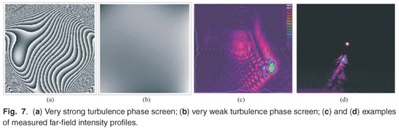
The phase change [Fig. 7(b)] at the lower end of the range is too small to record with the available grey-scale levels, since the full 256 levels are associated with a 2π phase shift. Thus again, the continuous phase function is written as a low-level binary element. The consequences of these deleterious effects can be seen in Figs 7(c) and (d): in the former, the additional energy in the various diffraction orders, due to the binary effects of SLM resolution, are noticeable; in the latter case, the zeroth order is very evident, indicating the low diffraction efficiency of the SLM under these conditions [note that Figs 7(a) and (c) do not form a pair, and likewise, (b) and (d)]. Further limitations include the frame rate of the SLM for time evolving turbulence, placing restrictions on the input parameters to the model, such as wind speed.
In order to quantify some of the effects noted above, consider that the efficiency of the SLM in producing the desired turbulence output in the m-th order is given by

with the energy distributed in discrete orders given by m = pN + 1 (for integer p), with N the number of pixels used in describing the phase between zones. Figure 8 shows a strong turbulence screen with example cross sections showing the phase modulation (0 – 2π) and the corresponding zones. The figure highlights that the zone spacing is not uniform across the SLM, and in this case, the spacing between zones decreases towards the edges of the SLM.

To illustrate the impact of this, we calculate the effective efficiency of the phase screens of Figs 8(b) and (c) as written to the SLM, assuming for convenience that the phase screens are written across 1000 pixels. The results are shown graphically in Figs 9(a) and (b), respectively.


The zone spacing in the horizontal cross section [Fig. 9(a)] is limited to only a few pixels near the edge, which decreases the efficiency in the 1st order to about 88%. The varying efficiency across the element leads to an effective amplitude mask that needs to be included in all calculations. In contrast, Fig. 9(b) shows high efficiency across the entire phase screen due to the large zone spacing. Note that these calculations are based on the phases shown in Figs 8(b) and (c), which we treat as independent functions in this analysis, in order to illustrate the SLM limitation better. When the turbulence is further increased, with D = 5.7 mm and r0 = 0.0001 m, the SLM is reduced to single pixel representation of each zone, thus resulting in either zero diffraction efficiency or zone shifting in a two-level element—both are undesirable.
When the turbulence is weak (D = 5.7 mm and r0 = 0.1 m), the SLM is still capable of resolving the small phase changes at about 5 pixels, giving >80% efficiency. As the turbulence is further decreased, so the number of pixels used will decrease, until the SLM displays a single-phase change across the entire beam, at the limit of very weak turbulence.
Conclusion
This work has outlined the basic steps required to simulate atmospheric turbulence in the laboratory using a spatial light modulator. The atmospheric model was collapsed into a single plane of turbulence of any desired strength, and implemented as a phase-only screen on the spatial light modulator. A Fourier-transforming lens allowed the far-field intensity pattern to be observed, so that any total propagation distance may be simulated.In order to simulate long-path turbulent atmospheres, one would require multiple phase screens to depict the turbulence; this could readily be implemented in the laboratory using multiple SLMs in series. We have highlighted some of the limitations in using SLMs for this application; these manifest themselves only at very strong and very weak turbulence as binary grating-like errors on the desired phase. We believe that this approach of using SLMs for the simulation of turbulence is versatile and cost-effective, and allows for useful laboratory-scale demonstrations.
1. Andrews L.C. and Phillips R.L. (1998). In Laser Beam Propagation Through Random Media. SPIE Optical Engineering Press, Bellingham, WA. [ Links ]
2. Andrews L.C. (2004). In Field Guide to Atmospheric Optics. SPIE Optical Engineering Press, Bellingham, WA. [ Links ]
3. Love G.D. et al. (1995). Binary adaptive optics: atmospheric wavefront correction with a half-wave phase shifter. Appl. Opt. 34, 6058–6066. [ Links ]
4. Love G.D. and Gourlay J. (1996). Intensity-only modulation for atmospheric scintillation correction by liquid-crystal spatial light modulators. Opt. Lett. 21, 1496–1498. [ Links ]
5. Love G.D. (1997). Wavefront correction and production of Zernike modes with a liquid crystal spatial light modulator. Appl. Opt. 36, 1517–1524. [ Links ]
6. Bold G.T., Barnes T.H., Gourlay J., Sharples R.R. and Haskell T.G. (1998). Practical issues for the use of spatial light modulators in adaptive optics. Opt. Commun. 148, 323–330. [ Links ]
7. Dayton D.C., Browne S.L., Sandven S.P., Gondlewski J.D. and Kudryashov A.V. (1998). Theory and laboratory demonstrations on the use of a nematic liquid crystal phase modulator for controlled turbulence generation and adaptive optics. Appl. Opt. 37, 5579–5589. [ Links ]
8. Noll R.J. (1976). Zernike polynomials and atmospheric turbulence. J. Opt. Soc. Am. 63, 207–211. [ Links ]
Received 22 January. Accepted 14 April 2008.
* Author for correspondence. E-mail: aforbes1@csir.co.za
The Zernike polynomials are a set of orthogonal polynomials that arise in the expansion of a wavefront function for optical systems with circular pupils. If we assume that the pupil is of unit radius, then the expansion of an arbitrary function ø(ρ, θ), where ρ∈[0, 1] and θ∈[0, 2π], in an infinite series of these polynomials, will be complete. The circle polynomials of Zernike have the form of complex angular function modulated by a real radial polynomial:

where n > |m|, n > 0 and n – m is even.
It can be shown that the radial function also obeys an orthogonality relation, and is given by

The radial function is normalized such that (1) = 1. By definition, when n – m ≠ even. Equation (A1) can be written as

thus we can construct two real functions  and
and  such that

where

The orthogonal property of these polynomials allows any function ø(ρ, θ) to be expressed as a linear sum of Unm and Vnm with suitable weighting coefficients Anm and Bnm, respectively, to yield:


