RESEARCH ARTICLES

 

Decomposing populations

 

 

P.G.L. Leach^{I, *}; K. Andriopoulos^II

^ISchool of Mathematical Sciences, University of KwaZulu-Natal, Howard College, Durban 4041, South Africa
^IIDepartment of Information and Communication Systems Engineering, University of the Aegean, Karlovassi 83 200, Greece

 

 

---

ABSTRACT

A decomposed system of differential equations is one which can be conflated into a single scalar equation in one dependent variable that contains all of the dependent variables of the original system. We consider the first-order differential equations for four standard models of population growth and give examples chosen from a variety of applications. We also present methods of analysis for integrable systems.

---

 

 

Models of population growth

There are several standard models for the rate of change of a population which we consider sufficiently large to be treated as a continuum, that is, the models which we use are based on ordinary differential equations rather than being discrete or stochastic models. They are

1.

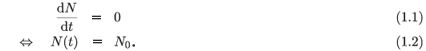
This is the trivial model in that the population is assumed to be constant. Such a model is not without its uses. If one is considering a population over a period of time sufficiently small for the normal means of increase and decrease of population to have any effect, one can treat the population as a constant. In one of the classical epidemiology models, the famous SIR model of Kermack and McKendrick,¹ described by the system of three equations

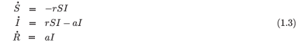
in which the overdot denotes differentiation with respect to time, the population N is divided into three groups, or compartments, comprising the susceptibles (S), the infectives (I) and the removed (R) we have such a situation. The contraction of the disease is measured at a rate r and is assumed to be proportional to the product of the susceptibles and the infectives, i.e. there is an assumption of the equal probability of mixing of any pairs in the population. Murray (ref. 2, p. 320) notes that this is a major assumption and in many situations does not hold, a notable example being most sexually transmitted diseases. The effect of the disease is measured by the rate of removal of infectives. In the case of a benign disease, this class becomes the proportion of the population which has recovered with immunity. In the case of a malign disease, this class is just the removed. Provided the disease acts over a short period of time, the constancy of the population may be assumed. In the case of a fatal disease, the shortness of the period of time is doubtless beneficial to the comfort of the investigators.

2.

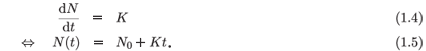
The constant rate of increase of the population described by (1.4) enables one to do a little more than with (1.1) without a serious increase in the mathematical difficulty.

3.

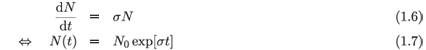
in which the proportional rate of change of population is given by the parameter σ. This is the famous model published by the Englishman, Thomas Malthus,³ in 1798 with the rather disconcerting implication that the continued rapid growth of population—a feature of 18th-century Europe by comparison with previous centuries during which plague and war effected a more modest rate of growth of population—would lead to massive starvation. The model excited public opinion and became sufficiently entrenched in the popular imagination for Malthus generally to be regarded as the pioneer of mathematical modelling in the inexact sciences, despite the rather more sophisticated model advanced by Daniel Bernoulli⁴ in his study of the effect of inoculation with cowpox on the spread of smallpox nearly 40 years before the work of Malthus was published. An integrable example of this nature has been discussed by Nucci and Leach,⁵ with the model described by the sets of equations

in which S(t) is the susceptible component of the population, I(t) is the infected component of the population, µK represents a constant rate of replenishment of susceptibles, µ is the proportionate death rate, β is the infectivity coefficient of the typical interaction term, and γ the recovery coefficient.

4.

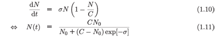
in which the additional parameter, C, is of the nature of a 'carrying capacity'. This variation was introduced 40 years after the model of Malthus in 1838 by the Hollander Verhulst,⁶ to avoid the obvious excesses to which the model of Malthus led. By a curious twist of fate (1.10), which is usually known as the logistic equation rather than Verhulst's equation, gained considerable notoriety about quarter of a century ago in its discrete form as a simple paradigm of chaos for suitable values of a parameter which is equivalent to the increasing of the time step to something considerably beyond a value which would be regarded as reasonable for a numerical procedure.

These four model equations—(1.1), (1.4), (1.6) and (1.10)—can be regarded as successive approximations of the same phenomenon. For a short period, one could regard the population as constant. For a longer period of time a constant rate of increase could be used. The next model is to assume that the rate is proportional to the existing population and, finally, one must take into account the limitations of the environment in which the population is growing by adding the additional term due to Verhulst.

Because these different models have validity for different regimes, it is possible to find a mixture of growth rates in a population containing varied components. An early example of this can be found in extensions to the models of Lotka and Volterra. Volterra⁷ proposed the model, related to fishing in the Adriatic,

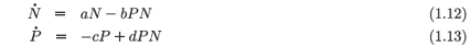
in which now N(t) is the population of the desired species (presumably desired for fishing) and P(t) is the population of a predator species. The parameters a, b, c and d determine the rates at which the populations increase and decrease and interact with each other. A similar model, in this case connected to chemical reactions, was proposed by Lotka⁸ about the same time. The bilinear term PN is typical of Lotka-Volterra models. In this model, the species N, the prey, is taken to have Malthusian growth with the implicit assumption that the species P, the predator, consumes sufficient of the prey for the Malthusian growth not to be excessive in terms of the carrying capacity of the local environment. In the case that the predator does not make serious incursions upon the population of the prey, it is more appropriate to replace the Malthusian term with a logistic term, so that (1.12) becomes

One notes that the Malthusian term in (1.13) gives a reduction in the population of the predatory species and so there is no need to introduce a logistic term here. Thus, in the one model different modes of growth of a population may be included without any affront to sensibility.

We further remark that these four model equations—(1.1), (1.4), (1.6) and (1.10)—are integrable, indeed trivially so. In fact all possess the Painlevé property, i.e. they have solutions in terms of analytic functions. We observe that the systems (1.3) and the pair (1.8) and (1.9) have the property that their respective sums are simply (1.1) and (1.4) in suitable variables, respectively. This is not the case with the Lotka-Volterra model, (1.12) and (1.13), except for the specific cases in which the parameters are related according to a = c and b = d and then the base model is simply (1.1).

Systems such as the SIR model represented by (1.3), which can be summed to give a single scalar equation in one variable, are called 'decomposed systems' and may be viewed as the decomposition of the single equation, (1.1) in the case of (1.3), according to some rule. The question which we wish to address here is the integrability of the decomposed systems.

We made the point above (following Murray²) that the assumption of free mixing is generally not valid for sexually transmitted diseases, but there is an example—based upon the properties of gonorrhoea—for which this occurs. The population is divided into two groups, male and female, and each of these two groups is divided into susceptibles and infectives. The argument is that a disease such as gonorrhoea does not confer immunity and so a person who has been treated returns to the class of susceptibles. The population is assumed to be constant in terms of the number of females and the number of males, so that the total population is also constant. The four-dimensional system is

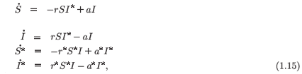
where the lower case letters are the rate constants and the symbols for susceptibles and infectives are obvious. For an unexplained reason, Murray (ref. 2, p. 329) makes the females the starred variables. We observe that (1.15) is a double decomposition in that we can write the basic system

as the two-dimensional system

where P = N + N*. Then each of (1.17) and (1.18) can be decomposed to give the system (1.15). However, the decompositions of (1.17) and (1.18) do not give two pairs of independent two-dimensional systems.

We are interested in integrable decomposed systems. It is important to realize that the general decomposition cannot be expected to be integrable. We consider an example which arises in an analysis of the Yang-Baxter equations,^9,10 but in reverse. The two-dimensional system

can be considered to be the decomposition of the Riccati equation

where z = r + w. The system (1.19) is integrable.¹¹ A further decomposition of (1.19), in fact to the form given by Golubchik and Sokolov,¹⁰ is

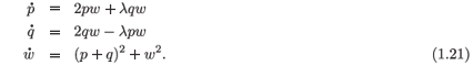
As a Riccati equation, (1.20) possesses the Painlevé property and is integrable in terms of analytic functions. The first decomposed system, (1.19), is equally well-integrable. The second decomposed system, (1.21), is, according to Golubchik and Sokolov, integrable, but this integrability is not in terms of analytic functions.¹¹

In this work we are concentrating on decomposible systems. More precisely, in the sequel we are going to address certain classes of decomposible systems. We accept that this is a restriction of the class of dynamical systems to be found in the analysis of various problems in epidemiology, ecology and related fields. However, we seek to explore the way in which integrable one-dimensional systems can be decomposed in such a way that the decomposed system is also integrable at the same level of integrability. Since our original systems—(1.1), (1.4), (1.6) and (1.10)—are integrable in terms of analytic functions, we look to analytic solutions for the decomposed systems.

A whole class of problems has been excluded from even the possibility of consideration in this work.

When we consider a population and its rate of change, the models which we have used, certainly in (1.6) and (1.10) as the rates of change in the two simpler models are independent of the population, look to the whole population as contributing to its increase or, as we have been considering the effects of disease or predation in the main, its decrease. In some populations, microbes come to mind; this is not unreasonable as microbes become capable of replication rather quickly. On the other hand, populations comprising more complicated species can be divided into the three classes of nonreproductive due to immaturity, reproductive and nonreproductive due to—may we politely put it—postmaturity. This class of population lies outside the class of decomposible systems considered in this work. Even models for which the concern of a proportion of the population being reproductive is not of major relevance can still exhibit the same problem. For example, in an epidemiological model for HIV infection in an homosexual population, Murray (ref. 2, p. 338) gives the system

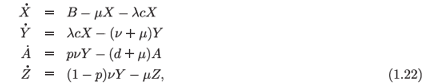
where X represents the number of susceptibles, Y the number of infectious HIV-positive persons, A the number of AIDS patients and Z the number of noninfectious HIV-positive persons. If we add the component equations of (1.22), we obtain the equation for the rate of change of the total population under consideration

where B represents the recruitment rate of susceptibles into the population, µ is the natural rate of demise and d the additional rate of demise of the AIDS-afflicted portion of the population, A. In the absence of AIDS, (1.23) would be a combination of the one-dimensional models (1.4) and (1.6). However, in the presence of AIDS the model (1.22) is without the bounds of consideration in this discussion.

 

Methods of analysis of systems of first-order ordinary differential equations

In the analysis of systems of first-order ordinary differential equations, which in general are not responsive to the ideals of integrability in terms of closed-form functions, the habit of almost a century, since the pioneering work of Poincaré established the power of his analysis, has been the analysis of the systems from the point of view of Dynamical Systems, which can be regarded as an outgrowth—a process of considerable generalization in itself—of the analysis of Hamiltonian systems in mechanics. In the fields such as ecology, economics, epidemiology and their likes the methods of Poincaré have been largely dominant for the simple reason that the systems of differential equations under investigation are rarely integrable in an 'obvious' fashionª). To the analytical methods of Dynamical Systems one can add the computational methods derived from numerical analysis. As long as the system has been established to be without chaos, one may rely upon the computations to provide a numerically accurate description of the evolution of the system. Of course, if the system is nonlinear—a not uncommon situation—in structure, the computation of solutions can be calculationally extremely expensive.

Somewhat neglected in the general scheme of these analyses are the two methods which have particular relevance to integrable systems. We refer to the symmetry analysis of Lie and the singularity analysis of Painlevé. We consider the latter first. The essence of the Painlevé approach is to expand the solution of the system of differential equations in terms of a Laurent series which contains a number of arbitrary constants equal to that of the order of the system. The precise details of the analysis may be found in such standard references as Ramani et al.¹² and Tabor.¹³

The symmetry analysis of Lie and its evolution over the past century and a quarter is simply a matter of invariance of a functional object.^b The invariance of a differential equation under a transformation—in principle finite, but the genius of Lie was to use the infinitesimal approach—has the effect of reducing the dimensionality of the extended phase space in which it exists and, if the number of symmetries being to both sufficient and of suitable nature,^c the differential equation is reduced to an algebraic equation and the system generated by the series of reductions rendered possible by the symmetries becomes a series of quadratures. This is integrability even though it may not be possible to express the solution in closed form.

In the analysis of the various systems presented below, we use the analyses of both Lie and Painlevé. The methods of symmetry analysis have become quite diverse over the years. In the first instance, the idea of a point or contact transformation, as is found in the works of Lie,^14-17 was extended to include generalized transformations by Noether¹⁸ and more recently to include nonlocal transformations.^9,20 The rationale for the extension of the type of symmetry—hence infinitesimal transformation and ultimately finite transformation—allowed can be stated to be simply one of utilitarianism.²¹ If one can make sense of the use of a particular symmetry in the solution of a system of differential equations, then that type of symmetry is useful. That these symmetries can fall outside the classical structure of Lie symmetries as representation of the classical Lie groups is not surprising. The classical Lie groups were established upon a certain structure and that structure was not as general as the types of symmetry considered now. There is in fact a pressing need for the re-establishment of the theory of Lie groups in terms of the modern appreciation of infinitesimal transformations related to differential equations. The reason for this is the important role which Lie groups have played in the interpretation of physical and other phenomena described by differential equations.

However, this is not the place for such an extensive discussion.

As the singularity analysis which is the essence of the Painlevé test is generally well known and the same can be said of the Lie analysis for symmetries, we give a brief explanation of the method of reduction of order,^22,23 with which the reader may not be so familiar.

 

The method of reduction of order

A system of differential equations

in which the element, x_j, of the multivariable, x, can occur in the right side as a derivative to an order of one less than the particular value of i in its peculiar differential equation, may always be written in terms of a system of first-order ordinary differential equations as

where we assume that the number of first-order equations equals the number of dependent variables by the simple device of defining the higher derivatives in (3.1) as new variables. Consequently, by a curious irony, in one sense, the method of reduction of order properly starts at (3.2). Since (3.2) is autonomous,^d one of the dependent variables may be chosen as a new independent variable. This is the standard method for the reduction of order of an autonomous system. For the sake of the presentation, we suppose that the chosen dependent variable is w_n. Then the system (3.2) may be replaced by

and we replace w_n by y to indicate its new status.

The analysis of a system, such as (3.3), of first-order ordinary differential equations for symmetries is a hazardous task as the system has an infinite number of symmetries and their determination is by a system of equations which requires the solution of the original system. One can make additional requirements upon the symmetries—an interesting and very useful requirement is mentioned in the section on the ladder problem—so that the process of determination is a somewhat more finite process than that of dealing with the infinite. One method to deal with this problem is to increase the order of some of the equations in the system of first-order equations (3.3). The process has been applied with singular success to the Kepler problem by Nucci²² in her demonstration that the complete symmetry group of the Kepler problem could be obtained by means of the standard methods of the Lie point symmetry analysis. A theoretical extension may be found in Nucci et al.²³ and a number of applications to variations on the basic underpinnings of the Kepler problem in Nucci et al.²⁴ One seeks to be able to solve the system of order (n - 1) for one of the dependent variables, so that it may be eliminated and in the process the order of at least one of the first-order differential equations be increased. In the case of a very agreeable system, this process may occur several times so that the system of n first-order equations may be considerably reduced in number. In principle this process could be used to reconstruct a single higher-order equation, but experience has shown that the extension of the procedure past second-order equations is no more productive than the reduction to second-order equations. Consequently, one looks to the reduction of (3.3) from a system of first-order equations to a system which involves at least one second-order equation. The intrusion of the second-order equation on the determination of the Lie point symmetries is extremely significant. The number of Lie point symmetries is reduced from infinity to a finite number, preferably a number not zero. The number of symmetries which can be determined from this system is frequently critical to the explanation, if not establishment, of the original system. We give a very simple example, albeit one which has attracted a literature of diverse opinion,^25-27,46 namely,

where p ≠ 0, 1, for which there exists not a single Lie point symmetry for general f. Nevertheless, (3.4) is obviously integrable.

 

The Ladder Problem

Our interest in decomposable systems arose from two papers by Imai and Hirata,^29,30 in which they developed a necessary condition for the existence of Lie point symmetries in n-dimensional systems of first-order ordinary differential equations and applied the ideas developed there to establish a new integrable family in the class of Lotka-Volterra systems.^e The Lotka-Volterra systems considered were quite specific in their structures. Both are homogeneous quadratic systems. The first system considered was called a ladder system because of the relationships between the elements of a matrix in the system. The ladder system is

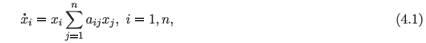
where the elements of (aij ) are defined by a_ij = i + 1 - j, i, j = 1, n. The generalized ladder system has a_ij = a₀ + a_i - a_j . The ladder system, which is always integrable in the sense of Lie, has been extensively investigated from the point of view of the Painlevé analysis by Andriopoulos et al.³¹ Imai and Hirata³⁰ established those values of the parameters in the generalized ladder problem for which integrability in the sense of Lie is found. We note that there is a spurious generality in the definition of the element for the generalized ladder problem, since the constant a₀ may always be rescaled to unity by means of a change of timescale.

In Andriopoulos et al.³² the starting point of the investigation was the observation that the ladder system is a decomposition of the one-dimensional Riccati equation

where the variable x is decomposed into x₁ + x₂ + … x_n. Equation (4.2) is decomposed according to the rule for (4.1), and the definition of a_ij for the ladder system of Imai and Hirata. Andriopoulos et al. considered the general problem of decomposition of the scalar autonomous Riccati equation

where the parameters A and B could take zero values as well as nonzero values.^f

 

Some illustrative examples

We consider three examples which illustrate these ideas for systems of the types = 0, = x and = x - x^2.

The classical S - I - R model

The classical model of Kermack and McKendrick¹ is described by the system

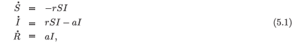
where in the context of epidemics S is the proportion of the population susceptible to the infection, I the proportion of population infected by the infection, and R that proportion of the population removed from consideration either through recovery or death. The parameters r and a represent the infection rate and the removal rate, respectively. The period under consideration is such that the normal means of entry and departure from the population may be ignored. One should emphasize that this model is not a priori a description of an epidemic. It is a description of a process of infection and removal. This may become an epidemic under what one could describe as inappropriate circumstances.

On the addition of the three equations comprising (5.1), we have

i.e. = 0, where now N = S + I + R. Obviously = 0 ⇒ N = constant = 1. Under the rescalings

the system (5.1) may be written in a form free of parameters as

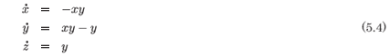
with the obvious summation (x + y + z)^. = 0.

The inclusion of the non-dominant term, -y of (5.4b), at the test for consistency shows that the system is not integrable in the sense of Painlevé. To overcome the problem of inconsistency at the resonance, a logarithmic term must be introduced.

The system (5.4) is a simple decomposition of an integrable scalar equation. Nevertheless it fails to be integrable in the sense of analytic functions. A suggestion of the problem is already found in the relationship between y and x, which can be determined from the integration of the ratio of (5.4b) and (5.4a), which gives

where A is the constant of integration. There may be a feeling of a sense of irony that one of the simplest of models in rational epidemiology does not have an analytic solution!

In the system (5.4) the variable z is ignorable and so the system is a candidate for the application of the technique of reduction of order developed by Nucci²² for the analysis of the Kepler Problem and elaborated by Nucci et al.²³ The quotients (5.4a)/ (5.4c) and (5.4b)/(5.4c) are

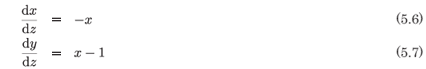
which is a system of one independent equation and one coupled equation. We note that the addition of these two equations and their subsequent integration leads to the conservation of the total population. In the spirit of the method of reduction of order, we would convert the system (5.6) and (5.7) to a single equation of the second order. We eliminate x to obtain

which is a linear quasi-first-order ordinary differential equation in y(z). From the solution of (5.8) we obtain the solution of the system (5.6) and (5.7) to be

so that (5.4c) becomes

The quadrature of (5.11) in closed-form is not possible.

We note that, as a linear second-order ordinary differential equation, (5.8) has eight Lie point symmetries (ref. 33, p. 405).

Tuberculosis and dengue fever

The techniques of the Lie symmetry analysis and the Painlevé singularity analysis have been applied to the simplified multistrain/two-stream models for tuberculosis and dengue fever, developed respectively by Castillo-Chavez and Feng³⁴ and Feng and Velasco-Hernández³⁵ and unified by van den Driessche and Watmough,³⁶ and by Nucci et al.³⁷ We use the form presented by van den Driessche and Watmough, namely

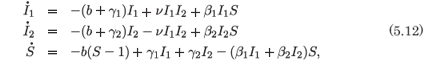
where β₁ and β₂ represent the infection rates for the two strains in the case of the tuberculosis model and for the two vectors in the dengue fever model, ν is the contact rate for a double dose of infection, b is the common birth and death rate, and γ₁ and γ₂ the recovery rates. The model, (5.12), does not represent the full system for the tuberculosis model,³⁴ but is a caricature of it to enable a common discussion with the dengue fever model.³⁵ The model has a single class of susceptibles and two classes of infectives corresponding to the two agents of infection.

The model (5.12) is a decomposition of

and belongs to the scheme of our discussion if we set W = N - 1 and T = bt, so that

There is equilibrium at W = 0, which corresponds to N = 1, i.e. constant demography.^g

A simplified model for gonorrhoea

At the outset we introduced a model—somewhat simplified we are informed—for the sexually transmitted disease gonorrhoea as presented by Murray.² We recall the set of equations as

and observe that not only is the total population preserved [see (1.16)] but also the populations of males and females separately in that we have

where N = S + I and N* = S* + I* and S and S* represent the susceptibles and I and I* the infectives of the male and female populations, respectively.

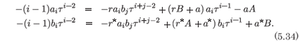
It is a simple matter to determine that the leading order behaviour is given by

and that the resonances occur at -1 and 1(3). We check for consistency at the resonance by substituting

into the full system (5.15) with the leading order terms as given in (5.18). At the resonance +1 we obtain the system

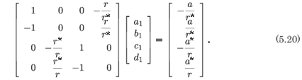
The system (5.20) can be written in a simpler form if the row operations = R₂ + R₁ and = R₄ + R₃ are performed. Then we have

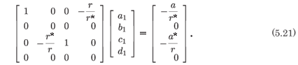
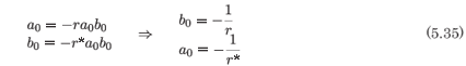
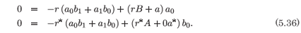
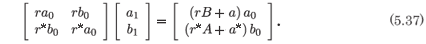
The consistency of the system is evident from (5.21). We note that the ranks of the coefficient matrix and the augmented matrix are both two and that we have the explicit relations

There are two arbitrary constants introduced at the resonance, i.e. the geometric multiplicity of the eigenvector is two. However, the resonance at +1 is a triple root, i.e. the algebraic multiplicity of the eigenvalue is three. There are only three arbitrary constants, the two introduced in (5.22) and the location of the movable pole, and so the solution presented cannot be the general solution of the system (5.15). To obtain the general solution one must introduce a logarithmic term and this destroys the analytic nature of the solution.

To make our analysis of the system (5.15) complete, we consider the transformation of the system of first-order equations to a scalar higher-order equation. Equations (5.16) and (5.17) are trivially integrated to give

where A and B are the values of the integrals of (5.16) and (5.17). We substitute (5.23) into (5.15b) and (5.15d) to obtain the system

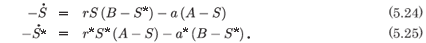
From (5.24) we obtain

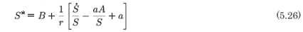
and, after we substitute this into (5.25) and make some rearrangements, we obtain the single second-order differential equation for S, namely,

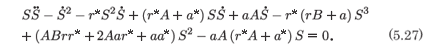
The first three terms in (5.27) are dominant and one is not surprised that the exponent of the leading order term is -1 and that the resonances are at ±1. We substitute

into (5.27) to establish that there is consistency at the exponent for which the resonance occurs. Specifically we obtain

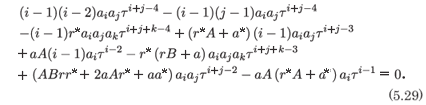
The coefficient of τ^-4 gives

and the coefficient of τ^-3 gives

From the result in (5.30) the coefficient of a₁ in (5.31) is identically zero as is to be expected as this is where the resonance occurs. The terms remaining in (5.31) give the condition

Subject to the constraint (5.32) on the parameters in (5.27), the latter equation has an analytic solution for S(t). It follows from (5.26) that S*(t) is also analytic and from (5.23) that I(t) and I*(t) are also analytic.

The existence of analytic solutions for both S(t) and S*(t) may explicitly be demonstrated by a performance of the Painlevé analysis on the system of first-order equations (5.24) and (5.25).

We make the substitutions

to obtain

From the coefficient of τ^-2 we obtain

and from the coefficient of τ^-1 we have

The rank of the coefficient matrix of the vector (a_1, b₁)^T is one. For consistency of the system we require that the coefficient of the augmented matrix also be one. This system is

The rank of this system is one if

which is precisely the condition we obtained from the analysis of the single second-order equation (5.27). We have the required two arbitrary constants and so there can be no question of the integrability of the first-order system given by (5.24) and (5.25). This analysis simply reinforces the conclusion reached above that the three-parameter solution obtained for the original system, (5.15), is analytic away from the movable polelike singularity. This type of integrability, which occurs for specific values of the first integrals of the base system determined by the relationship (5.38), is something of a generalization of the integrability which occurs when an integral takes a particular value, which is the case with configurational invariants^38,39 and in the case of the Painlevé analysis.^28,45 In the papers cited, the value of the first integral was quite specific whereas here it is a relationship between the values of two first integrals and this would represent a hypersurface in the space of initial conditions.

The solution obtained is not the general solution of (5.15), as it lacks the requisite four arbitrary constants of integration. However, by the procedure which has followed from the reduction of the system to a single second-order equation we have demonstrated the existence of an analytic solution of (5.15) containing three arbitrary constants of integration. Such solutions are not unknown. We already find one explicitly given in Ince's book (ref. 40, p. 355). Another explicit example is found in ref. 11, in which case the analytic solution of the system can be obtained in closed form by means of standard methods of integration. This type of solution has been interpreted⁴² as indicating that the system is at least integrable on a surface in the space of initial conditions. This interpretation is not universally accepted,⁴³ but in this instance the interpretation is based upon fact. One must agree that the interpretation has not been proven as a universal result.

The system (5.15) and the scalar equation (5.27) have the obvious Lie symmetry, ∂_t, reflecting their autonomy. Even with the constraint (5.32) there appears to be no other point symmetry. This is a little curious as one would expect some additional symmetry in the integrable case, compare similar instances in Nucci et al.⁵ and Torrisi and Nucci.⁴⁴ Evidently such additional symmetry is not of a point nature, but is either generalized or nonlocal.

Competition between species

To conclude our set of illustrative examples we consider the system

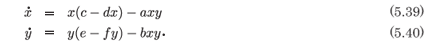
This can be taken as the system modelling two competing species. Both species have growth rates of logistic form and the competition is assumed to be proportional to the product of the two populations. To simplify the model so that we can easily treat it as a decomposed system, we assume that the parameters (c, d, e and f ) of the growth of population are sufficiently similar to be taken as equal. This would be the case, for example, of ruminants of similar reproductive habit, grazing the same area of grassland. Under this assumption we may rescale the independent and dependent variables so that the system contains just two essential parameters and may be written as

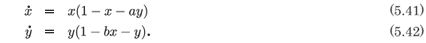
It is evident that the system (5.41, 5.42) is composible if a + b = 2, for then we have

where w = x + y.

For this model it is interesting to compare the results of the methods of analysis for integrable systems treated here with the information obtained by using the methods of dynamical systems. The equilibrium points of the system (5.41, 5.42) are located at (0, 0), (0, 1), (1, 0) and (x_e, y_e), where

Consistency of the system for the interior equilibrium point imposes the constraint that a = b = 1. In this case the point (x_e, y_e) is replaced by the line x_e + y_e = 1. The equilibrium point (0, 0) is unstable. Both equilibrium points (0, 1) and (1, 0) are saddles. In the case of (x_e, y_e) the eigenvalues are given by

The point is stable if the second eigenvalue is negative. However, if the system is to be composible, the second eigenvalue is necessarily positive and the point is a saddle.

We turn now to the singularity analysis of the system (5.41, 5.42). In general the coefficients of the leading-order terms are given by (5.44) and in the degenerate case β = 1 - α, which indicates that the nongeneric resonance in this case is zero. The resonances satisfy the equation

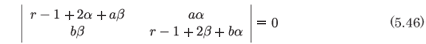
so that

and we note that the expressions for r coincide with those for λ in (5.45) above.

The system (5.41, 5.42) can possess the Painlevé property if a + b = n + 1 + ab(1 - n), where n is an integer. In the case that n = 1 we have the condition for the system to be composible and to have a saddle at the interior equilibrium point. However, we must check the full system for consistency with the behaviour of the dominant terms. When we substitute x = Σ_i=0 a_iτⁱ and y = Σ_i=0 b_iτⁱ into system (5.41, 5.42), we obtain

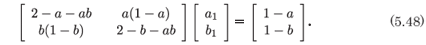
For consistency, the rank of the augmented matrix must also be one. This be the case if a + b = 2. As this is the condition for r = 1, we have consistency and the system possesses the Painlevé property.

One can, of course, examine the system for consistency with higher values of r. However, there is no possibility that the system (5.41, 5.42) is composible unless one has a = b = 1.

The composed system, (5.43), is a Riccati equation, a variables separable equation and a Bernoulli equation. We use of the third attribute to determine that

where A is the constant of integration. We substitute for y from (5.49) into (5.41) to obtain

where we have replaced the right side of (5.49) with F(t) to maintain a compactness of notation. The equation for x shares the same attributes as that for w. It has the solution

where B is the constant of integration and we have introduced 'new time' through the definition dT = (1 - aF )dt. The solution for y follows immediately.

This example contains some points of interest. In the case that the system (5.41, 5.42) is composible to the Riccati equation (5.43), there is a remarkable agreement in the main parameters of the singularity analysis and that of dynamical systems. Investigation of this feature in other systems could be of interest.

Time-dependent systems

It may have been observed that the systems treated above are autonomous. In the case of short timescales it is probably not unreasonable to assume that the parameters of a model are constant. However, on the longer timescales this is scarcely reasonable for many models. A simple example can be generated from the model of Volterra, (1.13) and (1.14), in reference to the problem of ruminants. In this case the prey comprises the grass and the predator the browser. Over the period of a year, the amount and quality of grass available to the grazing population varies. In a realistic modelling of the carrying capacity of a particular area, this variability in the amount of grazing available must be taken into account.

The same idea applies to many models. The treatment of time-dependent models is not as easy as that of autonomous models. One hopes that is self-evident. There is a technique available which enables one to combine the relative ease of treatment of an autonomous system with the greater accuracy of a time-dependent model. This is based in the Lie theory. Suppose that one obtains a certain set of symmetries for a given autonomous system, say by the method of reduction of order discussed above. Associated with these symmetries there is a Lie algebra,^h of which the given set of symmetries is a representation. One can look for other representations of the same algebra which do not include the symmetry of autonomy, namely, ∂_t, and so construct an equivalent system which is explicitly time-dependent. Such a system is as integrable as the original autonomous system. If the nature of the time dependence consistent with the algebra can be chosen to provide a reasonable replication of the variability of the parameters in the system one would expect over time, one has a much more useful model. Such a model could be used as the basis of a solution to provide a closer approximation to reality.

We give a simple example through an adaptation of the previous model for competing species. We observe that the condition for the system (5.41, 5.42) to be composible, namely, a + b = 2, does not require that a and b be constant parameters. Naturally, the ease of analysis by the approach of dynamical systems is lost and the singularity analysis becomes more complicated. Nevertheless, the composibility of the system and its integration are not seriously compromised. However, one may wonder a little about the underlying model. A more realistic model, in which the variation of the seasons affects the carrying capacity, is

where g(t) is some function which represents the variation of the seasons. The system (5.52, 5.53) is still composible if a + b = 2. There is still the potential for a and b to vary in time subject to this constraint. The composed system is

which is still a Riccati equation and a Bernoulli equation. The preferred route to integration is through the second option. We obtain

The equation for x is

and this is readily integrated to give

 

Conclusion

In this paper we have discussed a number of models arising in various contexts of population studies.

We have selected particular types of models being systems of first-order ordinary differential equations with the property that they can be conflated into a single scalar first-order ordinary differential equation in a variable which contains all of the dependent variables of the system. The composed equations were at most quadratic in the single dependent variable. Even in the case of the explicitly time-dependent model considered briefly as a final example, the integration of the single scalar equation was formally straightforward. The attraction of having a model which is the decomposition of a single equation is that the integration of that single equation gives a conservation law and so effectively reduces the order of the system by one. Indeed, the very existence of the scalar equation imposes a constraint and still reduces the order of a system by one.

Although we have treated models comprising only systems of first-order ordinary differential equations, the principle of composition can be further extended. There is no need for the equations to be of the first order. There is no need for the equations to be ordinary.

P.G.L.L. thanks the University of KwaZulu-Natal for its continuing support. K.A. thanks the State (Hellenic) Scholarship Foundation and the University of KwaZulu-Natal.

 

1. Kermack W.O. and McKendrick A.G. (1927). Contributions to the mathematical theory of epidemics. Proc. R. Soc. A 138, 55-83.        [ Links ]

2. Murray J.D. (2002). Mathematical Biology, I: An Introduction, 3rd edn. Springer-Verlag, New York.        [ Links ]

3. Malthus T.R. (1970). An Essay on the Principal of Population. Penguin, Harmondsworth.        [ Links ]

4. Bernoulli D. (1760). Essai d'une nouvelle analyse de la mortalité causée par la petite vérole, et des avantages de l'inoculation pour le prévenir. Histoire de l'Académie Royal des Sciences (Paris) avec Mémoires des Mathematiques et Physiques 1-45.        [ Links ]

5. Nucci M.C. and Leach P.G.L. (2003). An integrable SIS model. J. Math. Anal. Appl. 290, 506-518.        [ Links ]

6. Verhulst P.F. (1838). Notice sur le loi que la population suit dans son accroissement. Correspondences des Mathématiques et Physiques 10, 113-121.        [ Links ]

7. Volterra V. (1926). Variazione fluttuazione del numero d'individui in specie animali conviventi. Memoiri della Academia Linceinsis 2, 311-313.        [ Links ]

8. Lotka A.J. (1920). Undamped oscillations derived from the law of mass action. J. Am. Chem. Soc. 42, 1595-1599.        [ Links ]

9. Golubchik I.Z. and Sokolov VV. (1997). On some generalisations of the factorisation method. Theoret. Math. Phys. 110, 267-276.        [ Links ]

10. Golubchik I.Z. and Sokolov V.V. (2000). Operator Yang Baxter equations, integrable odes and nonassociative algebras. J. Nonlin. Math. Phys. 7, 184-197.        [ Links ]

11. Leach P.G.L., Cotsakis S. and Flessas G.P. (2000). Symmetry, singularity and integrability in complex dynamics: I The reduction problem. J. Nonlin. Math. Phys. 7, 445-479.        [ Links ]

12. Ramani A., Grammaticos B. and Bountis T. (1989). The Painlevé property and singularity analysis of integrable and nonintegrable systems. Phys. Rep. 180, 159-245.        [ Links ]

13. Tabor M. (1989). Chaos and Integrability in Nonlinear Dynamics. Wiley, New York.        [ Links ]

14. Lie Sophus (1970). Theorie der Transformationsgruppen: vol. I (reprinted: Chelsea, New York).        [ Links ]

15. Lie Sophus (1970). Theorie der Transformationsgruppen: vol. II (reprinted: Chelsea, New York).        [ Links ]

16. Lie Sophus (1970). Theorie der Transformationsgruppen: vol. III (reprinted: Chelsea, New York).        [ Links ]

17. Lie Sophus (1971). Continuerliche Gruppen (reprinted: Chelsea, New York).        [ Links ]

18. Noether E. (1918). Invariante Variationsprobleme. Küniglich Gesellschaft der Wissenschaften. Güttingen Nachrichten Mathematikphysik Klasse 2, 235-267.        [ Links ]

19. Abraham-Shrauner B. and Leach P.G.L. (1993). Hidden symmetries of nonlinear ordinary differential equations. In Exploiting Symmetry in Applied and Numerical Analysis, eds E. Allgower, K. Georg and R. Miranda (Lectures in Applied Mathematics 29, American Mathematical Society, Providence, RI) pp. 1-10.        [ Links ]

20. Géronimi C., Feix M.R. and Leach P.G.L. (2001). Exponential nonlocal symmetries and nonnormal reduction of order. J. Phys. A: Math. Gen. 34, 10109-10117.        [ Links ]

21. Govinder K.S. and Leach P.G.L. (1996). The nature and uses of symmetries of ordinary differential equations. S. Afr. J. Sci. 92, 23-28.        [ Links ]

22. Nucci M.C. (1996). The complete Kepler group can be derived by Lie group analysis. J. Math. Phys. 37, 1772-1775.        [ Links ]

23. Nucci M.C. and Leach P.G.L. (2000). The determination of nonlocal symmetries by the method of reduction of order. J. Math. Anal. Appl. 251, 871-884.        [ Links ]

24. Nucci M.C. and Leach P.G.L. (2001). The harmony in the Kepler and related problems. J. Math. Phys. 42, 746-764.        [ Links ]

25. González-Gascón F. and González-López A. (1988). Newtonian systems of differential equations integrable via quadratures, with trivial group of point symmetries. Phys. Lett. A 129, 153-156.        [ Links ]

26. Vawda F.E. (1994). An application of the Lie analysis to classical mechanics. Dissertation, University of the Witwatersrand, Johannesburg.        [ Links ]

27. Govinder K.S. and Leach P.G.L. (1997). A group theoretic approach to a class of second order ordinary differential equations not possessing Lie point symmetries. J. Phys. A 30, 2055-2068.        [ Links ]

28. Leach P.G.L., Nucci M.C. and Cotsakis S. (2001). Symmetry, singularities and integrability in complex dynamics V: Complete symmetry groups of nonintegrable ordinary differential equations. J. Nonlin. Math. Phys. 8, 475-490.        [ Links ]

29. Hirata Y. and Imai K. (2002). A necessary condition for existence of Lie symmetries in general systems of ordinary differential equations. J. Phys. Soc. Jpn 71, 2396-2400.        [ Links ]

30. Imai K. and Hirata Y. (2002). New integrable family in the n-dimensional heterogeneous Lotka -Volterra systems with Abelian Lie algebra. J. Phys. Soc. Jpn 72, 973-975.        [ Links ]

31. Andriopoulos K., Leach P.G.L. and Nucci M.C. (2003). The ladder problem: Painlevé integrability and explicit solution. J. Phys. A: Math. Gen. 36, 11257-11265.        [ Links ]

32. Andriopoulos K. and Leach P.G.L. (2003). Decomposition of the scalar autonomous Riccati equation (Preprint: Department of Information and Communication Systems Engineering, University of the Aegean, 83 200 Karlovassi, Grezce).        [ Links ]

33. Lie Sophus (1967). Differentialgleichungen (reprinted: Chelsea, New York).        [ Links ]

34. Castillo-Chavez C. and Feng Z. (1997). To treat or not to treat: the case of tuberculosis. J. Math. Biol. 35, 629-656.        [ Links ]

35. Feng Z. and Velasco Hernandez J.X. (1997). Competitive exclusion in a vector host model for the dengue fever. J. Math. Biol. 35, 523-544.        [ Links ]

36. van den Driessche P. and Watmough J. (2002). Reproduction numbers and subthreshold endemic equilibria for compartmental models of disease transmission. Math. Biosci. 180, 29-48.        [ Links ]

37. Nucci M.C. and Leach P.G.L. (2003). Tuberculosis and dengue fever: singularity and symmetry analyses of the simplified multistrain/two-stream models (Preprint: Dipartimento di Matematica, Università di Perugia, Perugia, Italy).        [ Links ]

38. Hall L.S. (1983). A theory of exact and approximate configurational invariants. Physica 8D, 90-105.        [ Links ]

39. Sarlet W., Leach P.G.L. and Cantrijn F. (1985). Exact versus configurational invariants and a weak form of complete integrability. Physica 17D, 87-98.        [ Links ]

40. Ince E.L. (1927). Ordinary Differential Equations. Longmans, Green, London.        [ Links ]

42. Cotsakis S. and Leach P.G.L. (1994). Painlevé analysis of the Mixmaster universe. J. Phys. A: Math. Gen. 27, 1625-1631.        [ Links ]

43. Contopoulos G., Grammaticos B. and Ramani A. (1994). The Mixmaster Universe revisited. J. Phys. A: Math. Gen. 27, 5357-5362.        [ Links ]

44. Torrisi V. and Nucci M.C. (2001). Application of Lie group analysis to a mathematical model which describes HIV transmission. In The Geometrical Study of Differential Equations (Contemporary Mathematics 285, American Mathematical Society, Providence, RI), 11-20.        [ Links ]

45. Richard A.C. (1995). Painlevé analysis and partial integrability of some dynamical systems. Dissertation, Department of Mathematics and Applied Mathematics, University of Natal, Durban.        [ Links ]

46. Abraham-Shrauner B., Govinder K.S. and Leach P.G.L. (1995). Integration of second order equations not possessing point symmetries. Phys. Lett. A 203, 169-174.        [ Links ]

 

 

Received 30 August 2005. Accepted 15 April 2006.

 

 

* Author for correspondence. E-mail: leachp@ukzn.ac.za; kand@aegean.gr
a Generally speaking, it is expected that these systems are integrable in the sense of being nonchaotic but nonintegrable in the sense of failing to possess a solution which can be expressed in closed form. It should be noted that 'closed form' does not carry the traditional implication of being expressible in terms of elementary functions. A closed-form solution can be in terms of special functions. The classic example of this is the equation + x = 0.
b Commonly this is considered to be a differential equation, but the idea is equally applicable to functions.
c The Lie symmetries of a differential equation constitute a Lie algebra and the internal relationships of the elements of the algebra act as possible constraints on their utility. For example, a differential equation invariant under a representation of the algebra so(3), the algebra of the rotation group in three dimensions has no further constraint imposed upon it by the third element of the algebra above those imposed by the first and second elements due to the cyclic nature of the Lie Brackets.
d The argumentation is equally valid for time-dependent systems since the time variable may be rendered dependent by means of the usual artificial choice of a new independent variable. For the purposes of the summary of the method presented in the body of this work, we assume that any adjustment has already been made before the analysis begins.
e Imai and Hirata imposed additional constraints upon the symmetries. In fact, the coefficient functions were required to be analytic in the neighbourhood of some fixed point and the symmetries were independent of time both in the coefficient functions and in the differential operators.
f An additional constant, say C, can be added to (4.3) if so desired and an equivalent analysis performed.
g Here we are being faithful to the representation of the models as given,^34,35 although, given the tendency towards mortality in both diseases and the absence of the politely termed 'removed' class, this does seem a little at odds with reality.
h There is no need to assume closure of the given symmetries. The additional symmetries required to close the algebra can be added to the set of symmetries determined from the analysis of the system. These additional symmetries are also symmetries of the system.