


Services on Demand
Article
 English (pdf)
 Article in xml format
 Article references
Indicators

Related links
-
 Cited by Google
 -
 Similars in Google
Share

 Permalink
South African Journal of Science
On-line version ISSN 1996-7489
Print version ISSN 0038-2353
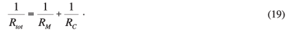
S. Afr. j. sci. vol.103 n.11-12 Pretoria Nov./Dec. 2007
RESEARCH ARTICLE
Cooling layers in rectangular heat-generating electronic regions for two boundary condition types: a comparison with a traditional approach
J. Dirker; J.P. Meyer†
Department of Mechanical and Aeronautical Engineering, University of Pretoria, Pretoria 0002, South Africa
ABSTRACT
This paper investigates the cooling ability of embedded solid-state, high-conductive layers in electronics applications. A numerical approach is used to determine and compare steady-state thermal characteristics of this internal heat transfer augmentation scheme for two thermal boundary condition types. The boundary conditions under investigation represent cases where a rectangular three-dimensional solid-state heat generating volume is externally cooled from its surface in either one or two orthogonal directions. Various material property and geometric parameters are considered. The numeric results are compared with predictions of a traditional planar conductivity approach. It is shown that a planar approach used for obtaining the thermal characteristics of a laminated composite structure over-simplifies the problem and only supplies an indication of the ultimate ideal cooling efficiency, which may be achieved, with cooling layers. This paper presents trends, which may be used to predict thermal characteristics more accurately for conditions where no thermal interfacial resistance is present.
Introduction
Innovative methods required to produce smaller electronic components, which operate at higher efficiencies and exhibit high levels of reliability, are becoming more crucial. This is especially true in, for instance, the power processing industry.1 A large obstacle regarding this is undesired heat production associated with energy losses occurring when any type of processing is performed. To maintain operating temperatures within acceptable ranges, the efficient removal of heat is of great importance and necessary for the future development of electronics.
Traditionally, externally mounted devices such as heat sinks (air cooled or liquid cooled) have been employed to reduce the thermal resistance between hot surfaces and the cooler environment. Owing to the improved transport of heat, lower operating peak temperatures in heat-producing devices can be achieved. Developments across almost the entire spectrum of electronics has required constant improvement of cooling methods to keep track with increased power densities.2 Other cooling methods include, amongst others, solid conduction cooling, liquid jet cooling, heat-pipe cooling, micro-channel cooling,14 evaporative cooling, and nucleation boiling cooling.3–5 Cooling techniques exhibiting high heat fluxes (W/m2), such as those making use of liquid to gas phase change, have played an important role and enjoy large research interest.
In certain applications as in passive power electronics, dominant thermal barriers are, however, not present on its external surface but within the structure of the device itself.6 Such passive power devices are responsible for electromagnetic energy storage and generally consist of materials with relatively low thermal conductivities such as ferrites.7 Thus, even though high heat fluxes can be attained on the exterior surface of such devices, the internal thermal resistance will ultimately determine internal peak temperatures of these components. In such cases the internal redesign of the devices could result in lower thermal resistance between known hotspots and the surface of the components.
Because almost all electronic components consist of solid-state materials, the optimization of heat transfer by internal conduction is a logical starting point for improving the thermal performance of structures with poor cooling characteristics. By introducing materials with relatively high thermal conductivities into the internal structures, thermal conduction paths can be created which conduct heat to surface regions, where it may be removed with conventional cooling methods.
In a previous investigation,8 it was found that the use of solid continuous internal cooling layers is a preferred means of improving thermal conduction from both a manufacturing and thermal performance viewpoint. The use of a tree-type configuration based on constructal theory9 has been suggested for optimum thermal performance. Such tree structures may prove difficult and expensive to manufacture. A more cost-effective alternative is the use of simplistic, continuous-embedded cooling layers.
New proposed configurations for integrated power electronic modules consisting of multiple materials sandwiched in a layered fashion10 is of special interest to this cooling enhancement alternative. Given the internal architecture of such proposed structures, it would be relatively easy to incorporate some form of internal cooling layer layout without significantly altering the electromagnetic function of the power electronics module. In an experimental study,11 it was found that the presence of ceramic aluminium nitride layers in ferrite was able to more than double the allowed power rating of the magnetic core under consideration for a given peak temperature.
Considering the cooling performances of highly conductive layers is not a new concept. It has long been realized that the copper layering on printed-circuit boards aids in the conductive cooling of these devices.12 Owing to the complex nature of heat flow patterns in such cases with multiple heat sources, rough estimations for equivalent planar and normal conductivity have been in common use. This is an over-simplification of the thermal conditions, however, and most likely leads to an underestimation of peak temperatures. Little in the literature deals with the cooling efficiency of embedded stacked cooling layers.
Purpose of the paper
In this paper the thermal performance of embedded internal cooling layers for a simplified uniform heat-generating volume is investigated numerically for conditions with repeating intermittent cooling and heat-generating layers. Under consideration are two types of thermal boundary conditions illustrated by means of the use of externally mounted heat sinks as shown in Fig. 1. In the one case heat is allowed to escape to the surroundings in one direction, whereas in the other case heat is released in two orthogonal directions. Numerical based results for these two boundary condition types are compared with each other as well as to results obtained using the traditional approach of defining an average equivalent thermal conductivity. The impact of thermal interfacial resistance will not be considered here, even though it plays a significant role.

Thermal modelling
Cooling-layer model problems representative of the two boundary conditions were defined as shown in Figs 2a and 2b. The model problems depict a composite heat-generating solid, which consists of alternating heat-generating and cooling layers. Cooling layers are orientated to promote heat transfer in either the z direction or both the x and z directions. The overall dimensions of the rectangular heat-generating solid in the x and z directions are 2A and 2Z, respectively. In the y direction, cooling layers are at a constant centre-to-centre offset distance of 2B, with each layer having a thickness of 2b. For both model types external heat transfer in the y direction was assumed to be insignificant in terms of the heat transfer associated in the other two directions. This assumption was made as there are no external heat transfer enhancement devices such as a heat sink or cold plate present on the upper and lower faces of the heat-generating structure.
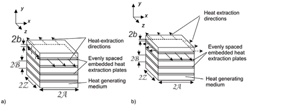

By considering the symmetric nature of the problem under investigation and the repetitive nature of the material layers, simplified thermal representative domains for each boundary condition can be defined as is shown in Figs 2c and 2d. The thermal behaviour of the layered structure can be investigated using these models. For the model problem where heat is allowed to escape to the surroundings from the device surface in only one Cartesian direction, a two-dimensional model was sufficient to investigate the temperature field. In this case no external heat transfer was allowed in the x direction. For the boundary condition case where external heat transfer is allowed in two orthogonal directions (in this example the x and z directions), a three-dimensional model was needed.
Provision is made for thermal interfacial resistance on all interfaces between neighbouring layers and on the external surface of the composite structure, where it is in contact with an external cooling device such as a heat sink. Adiabatic boundaries were defined on faces pointing towards the positive and negative y directions, the positive z direction and the positive x direction, where applicable.
The governing differential equation for the model problems within the layers (both heat generating and cooling) is given below.

Here T (K) represents temperature, k (W/mK) refers to thermal conductivity,  "' (W/m3) represents heat generation density within the heat-generating material, and x, y and z are the three Cartesian directions. Across an interface, the heat flux is defined as follows:

Here ΔT(K) refers to the temperature difference across the interface, R (m2K/W) represents the thermal interfacial resistance and " (W/m2) is the heat flux across the interface.
In the models the heat-generating medium and cooling layer material are referred to by subscripts M and C, respectively. Uniform internal interfacial thermal resistance between the heat-generating layers and cooling layers is represented by Rint (m2K/W), while external thermal resistance, where heat transfer to the surroundings is permitted, is represented by R ext (m2K/W). Adiabatic boundaries were defined by using the following equation (here direction x is used as an example):

The external surroundings were represented as an isothermal body having a reference temperature of T0. This body was not modelled. Of interest in this investigation was the relation between the heat-generation density and the peak steady-state operating temperature, Tmax. For the representative domains used in the two- and three-dimensional models, the location of this peak temperature is indicated in Figs 2c and 2d.
Solution approach
Owing to the discontinuities in material properties and thermal conditions at the interfaces between the different layers, a numeric solution to temperatures using Equation (1) could not be found. As result, a numeric solution approach was adopted. For both the two- and three-dimensional models, the representative domains were discretized into vertex-centred hexahedral elements.
In view of the simplicity of the representative domains, commercially available numerical software could easily have been used to obtain the temperature distribution within the regions of interest. However, as it was anticipated that an excessively large number of simulation runs would be required to fully investigate the thermal structures in terms of the dimensional parameters (A, b, B, Z), material property parameters (kM and kC), and interfacial parameters (Rint and Rext), problem-specific numeric algorithms were developed for the two model problems.
The main advantage of using such algorithms is that the time-consuming pre- and post-processing stages of numeric simulation with commercial packages could be automated. If simulation work had been performed using these packages, many fewer combinations of the input parameters could be considered in the time allowed.
Uniformly spaced node points were defined within the domains in either two or three directions as required by the model problem. The numerical algorithms made use of a fully implicit matrix-based solution approach to solve for the temperature value at each of these node points. Matrix bandwidth reduction techniques, such as the reverse Cutthill-McKee algorithm,13 were incorporated to reduce the computational time required.
Temperature solutions were tested for mesh independence by increasing the number of nodes defined within the domains and monitoring the change in the temperature values obtained. It was found that when more than 10 nodes were used in each Cartesian direction, the solutions obtained changed by less than 1% when the number of nodes in any direction was doubled. All subsequent simulations were conducted with 10 nodes in each direction.
Validation of numerical algorithms
The two-dimensional, single-directional numerical model was validated numerically with the use of the commercially available computational package, STAR-CD. A comparison of the temperature distributions obtained for an arbitrary case from the STAR-CD simulation result and that of the two-dimensional numerical model is shown in Fig. 3 along a nodal line in the y direction from point 2 to 1 as indicated in Fig. 2c. It was found that temperature values agreed within 0.1 K of each other. In addition to excellent numerical agreement, in a previous experimental study9 it was found that the two-dimensional model predicted relative thermal behaviour, for a single-directional surface heat extraction case, within 5%.

The three-dimensional model used for the two-directional external heat extraction boundary conditions was validated numerically by means of a commercially available computational package, Fluent version 6.1.22. A comparison of the temperature distributions obtained along an arbitrary nodal line in the y direction (from point 2 to point 1 indicated in Fig. 2d) is shown in Fig. 4. Good agreement was obtained between its results and those of a commercially available software package. Similar agreements were found for all validation runs conducted.

In addition to this, the solution obtained for the y–z view of the three-dimensional model on the adiabatic negative x face view was found to approach the y–z view solution of the two-dimensional model as A is increased. This is demonstrated for the case with and without thermal interfacial resistance in Fig. 5. The convergence to a two-dimensional temperature distribution as A is increased is expected because the thermal boundary condition on the positive x direction face has a reduced influence on the temperature distribution along line 1 to 2 (shown in Fig. 2d). In such cases, the temperature field on the negative x face can be obtained with the use of a two-dimensional model as was developed before.

From the validations described above, it was concluded that the problem-specific numeric algorithms developed could be used to investigate thermal behaviour and tendencies of embedded cooling layers.
Result processing
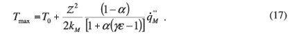
With the numerical models it was possible to relate the maximum temperature rise above the ambient, ΔTmax (K), to the volumetric heat-generation density in terms of a thermo-geometric coefficient, CGTP (W/m3K), for each test case:

From this it can be seen that higher CGTP values results in lower peak temperatures and better thermal performance. The effective volumetric heat-generation density increase at a fixed peak temperature, E%,eff (%), can be obtained by comparing the overall averaged heat-generation density of a volume consisting of a uniform heat-generating medium without cooling (reference case) and that of a volume which has cooling layers. This non-dimensional enhancement is defined as the percentage increase in the heat generation density that the composite volume containing cooling layers can accommodate while maintaining the original peak temperature [here α is defined as the volume fraction (b/B) occupied by cooling layers; subscript nc refers to cases with no cooling and subscript wc refers to cases with cooling]:
thus,
It should be noted that this increase is based on the overall global averaged heat-generation density, which includes the volume occupied by cooling layers, which in effect does not contribute to heat generation. The local heat-generation density within the heat-generating layers would therefore be greater than this average 'global' density.
For single-directional heat removal from a heat-generating medium without cooling layers, and Rext = 0 m2K/W, CGTP,nc can be obtained analytically by solving Equation (1) for one direction:

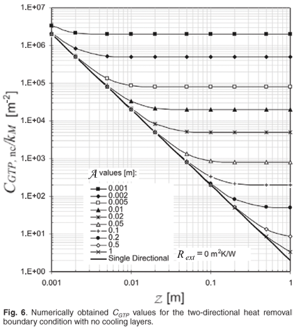
For two-directional heat removal without any cooling layers, Equation (1) has to be solved for two directions. For this boundary condition with Rext = 0 m2K/W, CGTP,nc is plotted in Fig. 5 in terms of some relevant values of A and Z. For comparison purposes, the CGTP values for the single-directional heat removal case is also indicated in the graph.
From this comparison it can be seen that CGTP values for two-directional heat removal are greater than or equal to CGTP for single-directional heat removal. As expected, and as is shown in Fig. 6, two-directional heat removal is thus more effective in reducing peak operating temperatures due to its exhibiting higher CGTP values. As an illustrative example, the CGTP,nc values for the two boundary conditions can be compared with each other for the case of a 20-mm square component (A = Z = 0.02 m). For single-directional heat removal, CGTP,nc has a value of 5000 whereas for two-directional heat removal it has a value of approximately 8000. By using Equation (4), it can be seen that a reduction of approximately 40% in the peak operating temperature may be expected if two-directional external heat removal is used instead of single-directional external heat removal.
When cooling layers are introduced for either boundary condition type, however, CGTP values are expected to increase, reflecting improved thermal performance.
Results
For cases where no internal or external thermal interfacial resistances are present, as is considered here, the non-dimensional cooling performance of a layered scheme, E%,eff was found to be dependent on parameter ratios and not necessarily on individual values of these parameters, as is discussed below. Such parameters include thermal conductivities and geometric dimensions.
As might be expected and also found, E%,eff is directly dependent on the geometric shape of the composite heat-generating structure expressed by two aspect ratios. The xz view (top view) shape of the structure can be described by dimensions A and Z or by the following ratio:

In addition to this, the proximity of cooling layers to each other can be expressed by their offset distance B, and one of their lengths (Z was chosen for this purposes in this paper) and combined to form the following ratio:

Another important aspect, as was highlighted earlier, is the proportion of the volume occupied by cooling layers, defined here again:

As with geometric shape, the thermal conductivity ratio obtained from the thermal conductivities of the heat-generating medium and cooling layer material also directly influence E%,eff. The following ratio was defined for this reason:

After completion of many numerical simulation runs, it was found that the non-dimensional cooling performance, E%,eff, is dependent on only the four ratios defined above (given that there is no thermal interfacial resistance). For the single-directional external heat removal boundary condition, E%,eff is dependent on α, γ and aZY, while for the two-directional external heat removal boundary conditionis E%,eff also dependent on aXZ (top view aspect ratio of heat-generating component). For cases with thermal interfacial resistance, these ratios alone are not sufficient to evaluate E%,eff.
The impact of the volume fraction, α, conductivity ratio, γ, and the proximity of cooling layers to each other, aZY, on E%,eff is indicated for single-directional external heat removal in Fig. 7. It can be seen that increases in any of these ratios improve the thermal enhancement of the structure. Identical trends for two-directional heat removal boundary case were exhibited for all simulation runs performed. The same was found to be true for the two-directional external heat removal boundary condition. An example of this boundary condition with α = 0.1 (10% of the total volume occupied by cooling layers) and γ = 20 for different top view aspect ratios of the composite structure is illustrated in Fig. 8.

From these figures it can be seen that as the number of cooling layers is increased and their thickness reduced in proportion (indicated by an increase in aZY), while maintaining a constant volume fraction α, E%,eff increases until it reaches an upper limit, E%,eff,max. Once this occurs, it is said that critical layer conditions have been reached.
Critical layer conditions
When the critical layer thickness has been reached, additional thermal advantage becomes insignificant when layer thickness is reduced further. For calculation purposes, critical layer conditions are reached when, by definition, E%,eff is within its upper 1% range. This can also be expressed by means of the following condition:

By studying the result given in Fig. 7, it can be seen that this maximum can be expressed as follows for the single-directional external heat removal boundary condition:

For the two-directional boundary condition, it can be seen from Fig. 8 that for four different values of aXZ (the top view xz aspect ratio of the composite heat-generating volume) E%,eff tends towards the same upper limit. It thus appears as if this upper limit is independent of the value of aXZ. After investigating various case studies, it was indeed found that this upper limit is dependent only upon the thermal conductivity ratio of the materials used, γ, and the fraction of the volume occupied by the cooling layers, α.
As with the single-directional boundary condition, an equation can be drawn up to describe this relation:

By comparing Equations (13) and (14) with each other, it is evident that very similar characteristics are present when considering the ultimate maximum thermal enhancement that can be achieved with the two boundary conditions. These equations are thus useful tools for determining E%,eff when cooling-layer thickness and offset distances are in the correct ranges.
By using the definition in Equation (6), these ranges for aZY were determined for both boundary condition types. The threshold value for critical layer conditions is indicated by  . If aZY > ZY, the use of Equations (13) and (14) becomes valid.
Threshold ZY values for the single-directional heat removal boundary condition is given for a wide range of α and γ in Fig. 9. The same type of information is given for the two-directional heat removal boundary condition in Fig. 10 for cases where aXZ = 1 (A = Z). For cases where A ≠ Z the threshold value of aZY needs to be adjusted according to the top view aspect ratio, aZY, as defined below:


Here, ζ is defined as an adjustment factor and is found to be dependent upon aXZ. ζ values can be read off in Fig. 11 for different aXZ values.

From Figs 9 and 10 it can be seen that, when cooling layers with relatively high thermal conductivities are used (high γ values), thinner layers are needed to reach the ultimate maximum E%,eff for the cooling layer material chosen. In terms of volume fraction, cooling layers are required to be at their thinnest for α = 0.5 (50% volume occupation) in order to reach ultimate E%,eff values predicted by Equations (13) and (14). Judging by the ZY values given, it can be seen that, in general, thinner layers (both heat-generating and cooling layers) are required when two-directional external heat removal is used than with the single-directional external heat removal.
Non-critical layer conditions
When manufacturing techniques do not allow for thin enough material layer thickness in order to reach the critical condition threshold, the thermal performance that can be expected will be reduced. The reduced E%,eff value can be expressed in terms of the maximum E%,eff value as follows:

with ε being a non-dimensional factor having a value of between 0 and 1.
Figure 12 demonstrates the dependence of ε upon α, γ and the ratio B/B*. Ratio B/B* serves as an indication of relative layer-thickness and offset-distance conditions in terms of the critical threshold. Here B* refers to the critical threshold half centre-to-centre offset distance between neighbouring cooling layers. If B/B* = 2 the layer thickness is twice that of the critical threshold layer thickness.

From the graph it can be observed that ε is not significantly affected by α when γ is greater than 30. Also, constant ε values are obtained for a wide range of γ values and it was found that for ratios of 2, 5 and 10, ε values in the regions of 0.95, 0.8 and 0.5, respectively, were obtained. This corresponds to E%,eff values of 95%, 80% and 50% of the ultimate E%,eff,max values. This means that if, for instance, layers were twice the thickness of that required to reach critical conditions, only about 5% of the ultimate thermal performance would have been lost. For five times the critical layer thickness, about 20% of the ultimate performance would be lost, and for ten times the critical layer thickness the loss would be about 50%.
Similar type graphs to that given in Fig. 12, which was created for single-directional heat removal, can be obtained for the two-directional boundary condition. In Fig. 13, ε values for this boundary condition is given for different top view aspect ratio of the composite heat-generating structure. Similar trends were obtained as with the single-directional external heat removal boundary condition. It seems as if α and aXZ have little impact on ε, and that only γ at low values (below about 30) has a significant influence on it.

With the information given above, a good indication can be obtained of the thermal characteristic of an embedded cooling-layer scheme for a wide range of geometric sizes and shapes and thermal conductivities. With some slight modification of the equations listed above, the following equations can be used to determine the peak maximum temperature within a composite layered structure.
For a single-directional external heat removal boundary condition:
For a two-directional external heat removal boundary condition:
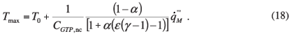
For the above equations, the values of ε and CGTP,nc need to be obtained from the relevant graphs given above.
Traditional planar thermal conductivity approach
When considering the two-layered configuration shown in Fig. 2c, the effective thermal conductivity can be determined according to the planar thermal conductivity approach,12 as discussed below. This approach is a common method used to analyse laminated structures thermally.
The total thermal resistance in the z direction is determined by considering each layer as a parallel thermal path:
For a length of Z and a unit depth in the x direction, the thermal resistance for each layer can be expressed as follows:

Substituting these, the following expression for the total thermal resistance can be obtained:

Comparing this to the thermal resistance of a single layer, the effective thermal conductivity in the z direction for the composite structure can be written as:

The analytical solution for the maximum peak temperature difference for one-directional heat removal without cooling layers being present is given below. This equation was obtained by integrating Equation (1) in one direction.

For the case with cooling layers and using the effective thermal conductivity obtained via the planar thermal approach discussed above, this equation can be written as follows by substituting in the effective thermal conductivity:

It should be noted that, due to the nature and origin of the above equation, "' already refers to the overall average heat generation density, which includes both the heat-generating and cooling material layers. With this in mind, the thermal performance increase can be written as follows (here subscript planar refers to the planar approached used above):

It can be seen that this equation is remarkably similar to the expressions derived earlier in this paper for the absolute maximum thermal performance. It should also be noted, however, that the planar approach is thus only valid to approximate the best thermal case when cooling performance has reached its maximum value, which can be achieved when layers are thin enough. When layers are not thin enough to be within the critical regions as reported on before, the use of this equation will result in under-prediction of the peak temperatures within a layered structure.
When using the local heat generation density in the heat-generating layers as reference, Equation (25) can be rewritten as follows (bearing in mind that 
It can be seen that Equations (17) and (18) bear a great resemblance to the one shown above. This acts as some form of verification for Equations (17) and (18). The main difference, however, is that Equation (27) does not take into account what the impact of layer thickness is, whereas those obtained from the numeric results do so via the inclusion of correction factor ε. This is specifically evident when comparing it to Equation (17), which is also derived for one-directional heat removal. The planar conduction theory does not consider the effect of thermal interfacial resistance on heat conduction phenomena. The impact of thermal resistance, which reduces thermal performance and increases peak operating temperatures, is not investigated here.
Conclusion
In this paper, equations were derived with which peak operating temperatures can be determined for a composite heat-generating structure consisting of alternating heat-generating and cooling layers. Two thermal boundary types were investigated numerically for conditions where no thermal interfacial resistance was present either internally between layers or on external surfaces. The thermal performance of an embedded layered scheme was found to be dependent on the fraction of the volume occupied by cooling layers and the ratio of the thermal conductivities of the cooling layers and the heat-generating layers. Correction factors that take into consideration the influence of layer thickness and the geometric shape of the composite structure for both boundary condition types, were determined for a wide range of thermal conductivities, and geometric dimensions. The equations derived from the numeric results were compared with an equation obtained using the more traditional planar conduction approach. We found that the planar conduction approach does not consider layer thickness and that peak temperatures will be under-predicted when this model is used.
Nomenclature
| aXZ | x–z view aspect ratio of heat-generating component |
| aZY | y–z view aspect ratio of rectangular region between the mid-plane surfaces of two adjacent cooling layers |
| CGTP | Coefficient dependent on geometric, thermal and material property values (W/m3K) |
| E%,eff | Effective thermal performance increase (%) |
| k | Thermal conductivity (W/mK) |
|
| Heat flux (W/m2) |
|
| Heat generation density (W/m3) |
| R | Interfacial thermal resistance (m2K/W) |
| T | Temperature (K) |
| x | Cartesian axis direction (m) |
| y | Cartesian axis direction (m) |
| z | Cartesian axis direction (m) |
| Greek and special characters | |
| α | Volume fraction ratio |
| A | Half x-directional dimension of heat-generating solid (m) |
| B | Half centre-to-centre offset distance in the y direction between cooling layers (m) |
| b | Half the width of cooling layer (m) |
| γ | Ratio of thermal conductivities of cooling layer and the heat-generating solid |
| ε | Correction factor for E%,eff taking layer thickness into consideration |
| ζ | Adjustment factor for critical layer threshold in terms of α and γ for the two-directional heat removal boundary condition |
| Z | Half z-directional dimension of heat-generating solid (m) |
| Subscripts | |
| ave | Average or global |
| C | Cooling layer |
| int | Internal interface between heat-generating material and cooling layer |
| ext | External interface of composite heat-generating component and heat sink |
| M | Heat-generating medium |
| max | Maximum (upper limit) |
| nc | No cooling |
| planar | Based on the planar conductivity approach |
| wc | With cooling |
| 0 | Ambient or reference |
| Superscript | |
| * | Critical layer conditions or threshold value. |
1. Van Wyk J.D., Strydom J.T., Zhao L. and Chen R. (2002). Review of the development of high density integrated technology for electromagnetic power passives. Proc. 2nd International Conference on Integrated Power Systems, pp. 25– 34. [ Links ]
2. Bergles A.E. (2003). Evolution of cooling technology for electrical, electronic, and microelectronic equipment. IEEE Trans. Components and Packaging Technologies 26(1), 6–15. [ Links ]
3. Murthy S.S., Joshi Y.K. and Nakayama W. (2002). Single chamber compact two-phase heat spreaders with microfabricated boiling enhancement structures. IEEE Trans. Components and Packaging Technologies 25(1), 156–163. [ Links ]
4. Kercher D.S., Lee J., Brand O., Allen M.G. and Glezer A. (2003). Microjet cooling devices for thermal management of electronics. IEEE Trans. Components and Packaging Technologies 26(2), 359–366. [ Links ]
5. Chien T., Lee D., Ding P., Chiu S. and Chen P. (2003). Disk-shaped miniature heat pipe (DMHP) with radiating micro grooves for a TO can laser diode package. IEEE Trans. Components and Packaging Technologies 26(3), 569–574. [ Links ]
6. Strydom J.T., Van Wyk J.D. and Ferreira J.A. (2001). Some units of integrated L-C-T modules at 1MHz. IEEE Trans. Industry Applications 37(3), 820–828. [ Links ]
7. Strydom J.T. and Van Wyk J.D. (2002). Electromagnetic design optimisation of planar integreted passive modules. Proc. 33rd IEEE Power Electronics Specialist Conference, Australia, 2, 573–578. [ Links ]
8. Dirker J., Malan A.G. and J.P. Meyer J.P. (2004). Numerical modelling and characterisation of the thermal behaviour of embedded rectangular cooling inserts in modern heat generating mediums. Proc. 3rd International Conference on Heat Transfer, Fluid Mechanics, and Thermodynamics (HEFAT 2004), Paper no. DJ1, Cape Town. [ Links ]
9. Almogbel M. and Bejan A. (2001). Constructal optimisation of nonuniformly distributed tree-shaped flow structures for conduction. Int. J. Heat Mass Transf. 44, 4185–4194. [ Links ]
10. Lee F.C., Van Wyk J.D., Boroyevich D., Jahns T., Chow T. and Barbosa P. (2002). Modularisation and integration as a future approach to power electronic systems. Proc. 2nd International Conference on Integrated Power Systems, pp. 9–18. [ Links ]
11. Dirker J., Liu W., Van Wyk J.D. and Meyer J.P. (2004). Evaluation of embedded heat extraction for high power density integrated electromagnetic power passives. Proc. Power Electronics Specialist Conference, Paper No. 11430, Aachen, Germany. [ Links ]
12. Yeh L-T. and Chu R. (2002). In Thermal Management of Microelectronic Equipment: Heat Transfer Theory, Analysis Methods, and Design Practices, pp. 177–180, ASME Press, New York. [ Links ]
13. Cerdán J., Marín J. and Martínez A. (2002). Polynomial preconditioners based on factorised sparse approximate inverses. Appl. Math. Comput. 133, 171–186. [ Links ]
14. Bello-Ochende T., Liebenberg L. and Meyer J.P. (2007). Constructual design: geometric optimization of micro-channel heat sinks. S. Afr. J. Sci. 103, 483–489. [ Links ]
Received 8 May 2006. Accepted 21 October 2007.
† Author for correspondence. E-mail: jmeyer@up.ac.za

