IUGG REPORTS

 

Recent research in geomagnetism and aeronomy in South Africa: 2003–2006

 

 

P.B. Kotzé

Hermanus Magnetic Observatory, P.O. Box 32, Hermanus 7200, South Africa. E-mail: pkotze@hmo.ac.za

 

 

---

ABSTRACT

This paper presents a brief review of research results from South African institutions on activities relating to the International Association of Geomagnetism and Aeronomy (IAGA) during the quadrennium 2003–2006. The institutions actively involved included: the School of Physics, University of KwaZulu-Natal, Durban; Hermanus Magnetic Observatory, National Research Foundation, Hermanus; the Department of Physics and Electronics, Rhodes University, Grahamstown; and the Unit for Space Physics, Department of Physics, North-West University, Potchefstroom. The article is organized according to the core activities of the IAGA.

---

 

 

Geomagnetism

Geomagnetic observatories, field surveys and modelling

Continuous recording of geomagnetic field variations are conducted at Hermanus (34°35.5'S, 19°13.5'E), Hartebeesthoek (25°52.9'S, 27°42.4'E) and Tsumeb (19°12'S, 17°35'E). All three observatories comply with INTERMAGNET standards. The primary instrument for recording magnetic field variations is the FGE fluxgate magnetometer, manufactured by the Danish Meteorological Institute in Copenhagen. This equipment is based on three-axis, linear-core fluxgate technology, optimized for long-term stability and records the components H, D and Z. An Overhauser-type magnetometer further provides absolute total field information, while baselines for the other components are obtained using a DI Flux theodolite.

For field survey purposes, field stations are marked by concrete beacons, ensuring that all observation points are exactly re-occupied during surveys. Most measurements are taken on a standard 1.2-m pillar, while in a few cases observers have to use a tripod mounted above a clearly marked shorter beacon.

The international and local geophysics communities have expressed much interest in the rapid decrease in the geomagnetic main field in the southern African region,¹ which suggests that a reverse dynamo may be developing below South Africa as observed by Hulot et al.² The Hermanus Magnetic Observatory (HMO) and the GeoForschungsZentrum (GFZ), Potsdam, Germany, have begun a collaboration to study this phenomenon using ground-based and satellite data. This combined project between Germany and South Africa, called Inkaba ye Africa, the COMPASS (for COmprehensive Magnetic Processes under the African Southern Sub-continent) programme, aims to study the geomagnetic field and in particular its evolutionary behaviour. In addition to the decline in the geomagnetic field in this region as evidenced by the 20% fall observed at Hermanus, the orientation of the geomagnetic field in southern Africa is also changing rapidly.³ In the northwestern part of the subcontinent, the declination of the magnetic field is propagating eastward (observed at Tsumeb) and westward in the southeastern part (noted at Hermanus and Hartebeesthoek). This results in the spatial gradient over the subcontinent increasing with time.

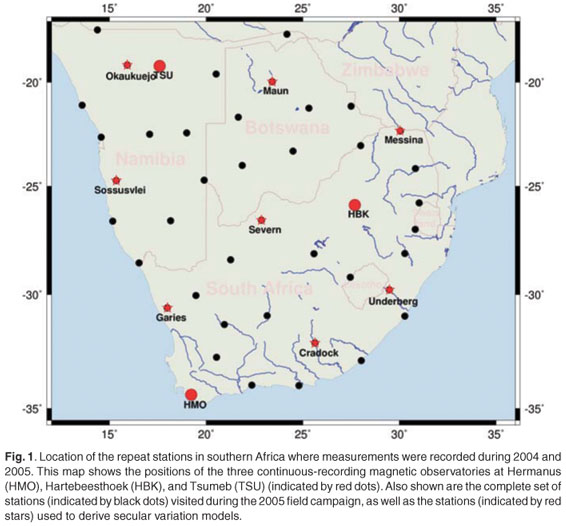
During 2005 and 2006, joint field survey campaigns were conducted by the HMO and the GFZ in South Africa, Namibia and Botswana, to characterize the variation with time of various components of the geomagnetic field. Two independent teams, each consisting of a staff member from HMO and GFZ, conducted a simultaneous field survey in southern Africa and visited the survey beacons indicated in Fig. 1. Some isolated repeat stations were found not to be suitable for field survey measurements. This was mostly because the region was not magnetically quiet, or that the observation pillar was destroyed by urban expansion. A DI fluxgate magnetometer was used as the primary instrument during field surveys, while an Overhauser magnetometer delivered values of total field intensity. Corrections for diurnal variation and other disturbing effects were made by comparing field station observations with magnetic data recorded on site with a LEMI suspended tri-axis fluxgate instrument.⁴ Referring to additional magnetic observatories, sometimes a distance of more than 300 km away, greatly improved the quality of the measurements. Results obtained from this survey, together with information acquired from a previous survey conducted in 2004 at eight field stations, as well as the data from the three continuous-recording observatories at Hermanus, Hartebeesthoek and Tsumeb, were used to model the geomagnetic-field time variation for 2004/5, employing a polynomial approach.⁵

 

 

As part of the collaboration between GFZ and HMO, instruments for a new magnetic observatory at Keetmanshoop in Namibia were installed at the local airport in late 2005.⁶ This location was specifically chosen to be about halfway between Hermanus in the south and Tsumeb in the north, to correct for disturbance effects from external sources and to refer the repeat station data to a common epoch during field surveys. This newly established INTERMAGNET-grade observatory will play a key role in the region, because: 1) It will serve as a reference magnetic observatory for field stations within a radius of 600 km, located in the large area between the Northern Cape and southern Namibia, a region which has not been adequately covered in the past. 2) It will be an accurate monitor of spatial changes in secular variation across southern Africa. The variations in the declination at the southeastern and northwestern borders of southern Africa are currently 11 arc min/yr westward and 6 arc min/yr eastward, respectively.¹ The Keetmanshoop observatory, located between Hermaus and Tsumeb in a north–south direction, as well as in an east–west direction on approximately the same magnetic latitude as Hartebeesthoek, will help accurately to monitor the spatial change of secular variation across southern Africa.

The latest field survey was conducted with logistical support from the Geological Survey of Namibia as well as from the Namibia Airports Company. The recording instruments, a 3-axis FGE fluxgate magnetometer, an Overhauser absolute magnetometer, as well as a DI Flux theodolite for taking absolute measurements, were provided by GFZ, while HMO contributed the glass-fibre box for housing the instruments. The design of this observatory is unique, as it deviates substantially from traditional recording equipment. The entire observatory is buried underground in the glass-fibre container, and then filled with water bottles for temperature stabilization. The data recording computer, with its cellphone technology for data transmission, were installed early in 2006. Data are currently transmitted to Hermanus on a daily basis, while baselines are determined at regular intervals by personnel at Keetmanshoop airport.

ULF geomagnetic pulsation data

The HMO continued to record ultralow-frequency geomagnetic pulsation data at Hermanus, and also at Sutherland (32°24'S, 20°40'E). The data were obtained by measuring the voltages induced in two horizontally mounted induction sensors, one orientated approximately in the magnetic meridian (H-component) and the other perpendicular to this direction (D-component). The data are logged digitally on a PC with sampling at 1-s intervals and accurate timing provided by a GPS receiver. The appearance of Pi2 pulsations in the data is used by researchers worldwide to determine the occurrence and timing of substorm onsets and enhancements.

 

Aeronomic phenomena

Total electron content mapping

The Grahamstown, South Africa (33.3°S, 26.5°E) ionospheric field station operates a UMass Lowell digital pulse ionospheric sounder (Digisonde) and an Ashtech geodetic grade dual-frequency GPS receiver. The GPS receiver is owned by the Chief Directorate Surveys and Mapping in Cape Town, forms part of the national TrigNet network and was installed in February 2005. The sampling rates of the GPS receiver and Digisonde were set to 1 second and 15 minutes, respectively. Data from four continuous months, March to June 2005 inclusive, were considered in this initial investigation. Data available from the Grahamstown GPS receiver were limited and, therefore, only these four months have been considered. Total electron content (TEC) values were determined from GPS measurements obtained from satellites passing near the vertical (within an 80° elevation) to the station. TEC values were obtained from ionograms recorded at times within 5 min of the near-vertical GPS measurement as reported by Cilliers et al.⁷ The GPS-derived TEC values are referred to as GTEC and the ionogram-derived TEC values as ITEC. The GTEC and ITEC values were compared, with the differential clock biases of the GPS satellites and receivers taken into account. The plasmaspheric contribution to the TEC could be inferred from the results, and confirmed findings obtained by other groups.

South Africa has three operational ionosondes, whose data have been used in developing a national model. The South African network of GPS receivers, as shown in Fig. 2, is expanding and the long-term plan is to use the data from these receivers to derive ionospheric information over the areas that are not covered by the current ionosondes. This will allow use of an existing network to supplement the ionospheric network, thereby providing a more comprehensive map of ionospheric behaviour over South Africa.

 

 

Neural network modelling of ionospheric parameters

Neural networks (NNs) are proving to be ideal tools for modelling the behaviour of the ionosphere. The NNs are trained using a database of archived data describing the relationship between the output parameter and an input space. The input space is designed from knowledge of those variables that affect the behaviour of the output parameter. For ionospheric parameters this input space includes a solar variable because of the strong influence of the Sun on ionospheric behaviour.

An investigation was conducted by Oyeyemi and Poole,⁸ using the critical frequency of the F2 layer, foF2, which provides an indication of the ionospheric maximum electron density, to demonstrate how NNs can be used to determine the optimum solar input variable for use in predicting foF2. Among the solar criteria used are the daily sunspot number, the F10.7-cm solar radio flux, and the solar irradiance. Varying time lengths of these parameters were also investigated. The criteria used in determining the optimum input is the root-mean-square (RMS) error between the measured and predicted output parameters.

The technique of neural networks⁹ has provided a powerful new method for developing models to predict and forecast the highly nonlinear behaviour of the ionosphere. In addition, NNs offer another means for determining the optimum input parameters required for the prediction of ionospheric parameters. The networks can also provide evidence of the existence and extent of new relationships between unknown geophysical parameters and the ionospheric output. Neural networks combine archived databases that record the history of ionospheric behaviour, the experience and expertise gained from years of analytical analysis and measurements, and the advanced computing power, skills and technologies of today, to give an all-in-one solution to a nonlinear problem.

Neural networks have been employed also to develop a global model of the foF2 frequency.¹⁰ The main principle behind this approach is the use of parameters other than simple geographic coordinates, on which foF2 is known to depend, and exploiting the ability of NNs to establish and model this nonlinear relationship for predictive purposes. The foF2 data used in the training of the networks were obtained from 59 ionospheric stations across the globe at various times from 1964 to 1986, on the basis of availability. To test the success of this approach, one neural network (NN1) was trained without data from 13 stations, selected for their geographic remoteness, which could then be used to validate the predictions of the NN for those remote coordinates. These stations were subsequently included in the final neural network (NN2). The input parameters consisted of day number (day of the year), universal time, solar activity, magnetic activity, geographic latitude, angle of meridian relative to subsolar point, magnetic dip angle, magnetic declination, and solar zenith angle. Comparisons between foF2 values determined using NNs and the International Reference Ionosphere (IRI) model [derived from Union Radio Scientifique Internationale (URSI) and International Radio Consultative Committee (CCIR) coefficients] with observed values are given with their RMS error differences for test stations. The results from NN2 are used to produce the global behaviour of hourly values of foF2 and are compared with the IRI model using URSI and CCIR coefficients. The RMS error differences obtained, which compare favourably with the IRI models, justify this technique for global foF2 modelling.

The neural network technique for the development of a near-real-time global foF2 (NRTNN) empirical model was used at Rhodes University by Oyeyemi et al.¹¹ The data used are hourly daily values of foF2 from 26 worldwide ionospheric stations (based on availability) during the period 1976–86 for training the network, and between 1977 and 1989 for verifying the accuracy of prediction. The training data set includes all periods of quiet and disturbed geomagnetic conditions. Two categories of input parameters were used as inputs to the NN. The first group consisted of geophysical parameters that were temporally or spatially related to the training stations. The second category, which was related to the foF2 itself, consisted of three recent past observations of foF2 9 (i.e. real-time foF2, and also 2 h and 1 h previously) from four control stations [namely, Boulder (40.01°N, 254.71°E), Grahamstown, Dourbes (50.11°N, 4.61°E) and Port Stanley (51.71°S, 302.21°E)]. The performance of the NRTNN was verified, under both geomagnetically quiet and disturbed conditions, with observed data from a few verification stations. The RMS error differences between measured values and the NRTNN predictions were compared with our earlier standard foF2 NN empirical model. They revealed that NRTNN will predict foF2 in near-real time with about 1 MHz RMS error difference anywhere on the globe, provided real-time data are available at the four control stations. It is also evident from these results that in addition to the geophysical information from any geographical location, recent past observations of foF2 from these control stations can be used as inputs to a neural network for near-real time foF2 predictions. Results also reveal that there is a temporal correlation between measured foF2 values at different locations.

The application of NNs was further extended by Oyeyemi et al.¹² to develop a global model of the ionospheric propagation factor M(3000)F2. Neural networks were trained with daily hourly values of M(3000)F2 from various ionospheric stations spanning the period from 1964 to 1986, with the following temporal and spatial input parameters: universal time, geographic latitude, magnetic inclination, magnetic declination, solar zenith angle, day of the year, A16 index (a 2-day running mean of the 3-hour planetary magnetic a_p index), R2 index (a 2-month running mean of sunspot number), and the angle of the meridian relative to the subsolar point. The performance of the NNs was verified by comparing the predicted values of M(3000)F2 with observations from a few selected ionospheric stations and the IRI model [CCIR M(3000)F2 model] predictions. The results obtained compared favourably with the IRI model and, from the error differences, justified the potential of the NN technique to predict M(3000)F2 values on a global scale.

Furthermore, a new neural network-based global empirical model for the F2 peak electron density has been developed by Oyeyami and McKinnell at Rhodes University, using extended temporal and spatial geophysical inputs. Ground-based ionosonde data from 80 global stations, spanning the period 1995 to 2005, and for a few stations from 1976 to 1986, and from various resources of the World Data Centre (WDC) archives [Space Physics Interactive Data Resource (SPIDR), the Digital Ionogram Database (DIDBase), and IPS Radio and Space Services] have been used for training a neural network. The training data set includes all periods of quiet and disturbed magnetic activity. Comparisons were then made of experimental observations and foF2 values predicted from the NN-based and IRI models, for all conditions (such as magnetic storms, levels of solar activity, season and different latitudes). The RMS error differences for a few selected stations were substantially improved over previous model results, demonstrating that this new model can be used as a replacement option for the URSI and CCIR maps within the IRI model for the purpose of predicting F2 peak electron densities.

Neural networks have recently been used also to model the ionospheric electron density profiles over both South Africa (LAM model) and at high latitudes. The NN-based Ionospheric Model for the Auroral Zone (IMAZ) was developed in a joint South African–Austrian effort to provide a reliable prediction tool for the electron density profile at altitudes below 150 km and at high latitudes. A combination of data obtained from the European Incoherent Scatter Radar (EISCAT) and measurements from rocket-borne wave propagation experiments provided enough high-latitude data to cover one solar cycle. The inputs to this model are local magnetic time, total absorption, local magnetic activity, solar zenith angle, and the F10.7-cm solar flux value. The pressure surface, which combines the effects of the seasonal variation and the altitude, is also included as an input parameter. The output is the electron density at the given input pressure (corresponding to altitude).

Both models provide realistic electron density profiles within the boundaries laid down by the data with which the NNs were trained and the purposes for which the models were developed. Predicted profiles from each model indicate that NNs provide a more successful approach to electron density profiling than analytical techniques.

Stratospheric studies

There were several large X-class solar flares and associated solar energetic particle (SEP) events during January 2005. Coincidentally, the MINIS balloon campaign had multiple payloads aloft in the stratosphere above Antarctica, measuring d.c. electric fields, conductivity and X-ray flux. One-to-one increases in the electrical conductivity and decreases to near zero of both the vertical and horizontal electric field components, in conjunction with an increase in particle flux at SEP onset, were observed by researchers from the University of KwaZulu-Natal and elsewhere, and were reported by Kokorowski et al.¹³ Combined with an atmospheric electric field mapping model, these data are consistent with a shorting out of the global electric circuit and point towards substantial ionospheric convection modifications. Two subsequent, rapid changes were detected in addition in the vertical electric field component several hours after SEP onset. These changes result in similar fluctuations in the calculated vertical current density.

From the MINIS observations, it is evident that the SEP event of 20 January 2005 had a significant impact on atmospheric electrodynamics. Although the MINIS observations are consistent with previous measurements, deviations from them were also observed. Previous in situ measurements described a sudden decrease in the magnitude of the vertical electric field and conductivity enhancement coinciding with the onset of an SEP event. The MINIS data are consistent with this basic observation. What sets the MINIS data apart are the two subsequent, rapid jumps in the d.c. vertical field several hours afterwards and the observations of the total (not just vertical) electric field disappearing suddenly at SEP onset. These two unique features of the MINIS data set cannot be explained by simply enhancing the atmospheric conductivity. Rather, it is likely that the rapid vertical fluctuations are related to rigidity cutoff motion, while the vanishing of the horizontal field may be connected to magnetospheric dynamics.

 

Magnetospheric phenomena

Cosmic radio noise absorption and auroral luminosity studies

Cosmic radio waves of 5–10-m wavelengths recorded by the riometers at the South African Antarctic base SANAE IV at Vesleskarvet have been used to investigate ionization structures in the ionosphere. In related studies, the structures in riometer absorption were compared with digitized all-sky images of auroral optical emissions recorded by a low-light-level TV system. Stoker et al.¹⁴ digitized all-sky images of auroral optical emissions, recorded at SANAE IV (70.3°S, 2.4°W, L = 4.0), and then mapped them onto the angular sensitivity functions of both a broad, single-beam riometer and the narrow beams of an imaging riometer.

Observations during a substorm expansive phase at SANAE IV showed that the 630.0-nm auroral spectral line closely followed the variations in the auroral white light (mainly green and blue spectral lines), and preceded the white light variations from about 0 to 5 s during the observation of a pre-midnight substorm on 19 July 2003. Absorptions in cosmic radio noise appeared to vary in a way both related and unrelated to optical emissions. Associated variations were delayed relative to optical variations from 2 to 12 s. These temporal differences in variations support the idea of a local dispersionless acceleration region associated with the expansion phase of the substorm. The temporal differences suggest an increasing electric field as an acceleration mechanism. The unrelated absorptions in cosmic radio noise had then to originate from a different acceleration region.

Studies of Pi2 pulsations

It is well known that Pi2 pulsations, which are impulsive, strongly damped, ultra-low-frequency oscillations of the geomagnetic field, occur at the time of magnetospheric substorm onsets and intensifications. Pi2 pulsations recorded at low latitudes in particular, where amplitudes typically lie in the range 0.25–2.5 nT, are one of the clearest indicators of substorm onsets. The HMO has played an important role in studies carried out at local and foreign institutions to gain a better understanding of the dynamics of the earth's plasma sheet. The observatory's contribution has been to provide and analyse low-latitude, ground-based ULF pulsation data, primarily on Pi2 pulsations.

Nosé et al.¹⁵ investigated a Pi2 pulsation that occurred at 05:38 UT on 20 September 1995, using data from ground stations and the ETS-VI and EXOS-D satellites. Because ground stations at L = 1.45_12.6 and the two satellites were located at 7–10 hours of magnetic local time (MLT), they could investigate characteristics of the morning-side Pi2 pulsation in detail. They also examined geomagnetic field data from equatorial and low-latitude (L_1.5) stations at 02:00 MLT and 15:00 MLT. Their findings included the following: (1) Pi2 pulsations on the morning side were observed over a wide range of L (L < 6.1) with almost identical period (T_70 s) and waveforms; (2) the ETS-VI satellite located above the geomagnetic equator at L = 6.3 observed a Pi2 pulsation that had nearly the same period and waveforms as the ground Pi2 pulsation; (3) the Pi2 pulsation observed by ETS-VI appeared in the compressional and radial components; (4) the EXOS-D observation placed the plasmapause location at L = 6.8, across which ground Pi2 pulsations changed their characteristics; and (5) no phase delay was found between low-latitude Pi2 pulsations observed around 07:00, 02:00, and 15:00 MLT. They therefore concluded that the morning-side Pi2 pulsation was caused by the plasmaspheric cavity mode resonance and that its longitudinal structure was relatively uniform.

Further studies by Nosé et al.¹⁶ on the longitudinal characteristics of Pi2 pulsations revealed the longitudinal structure of the plasmaspheric cavity mode. They used the geomagnetic field data from two ground stations, at Kakioka (27.2° geomagnetic latitude, 208.5° geomagnetic longitude) and Hermanus (_33.9° geomagnetic latitude, 82.2° geomagnetic longitude), and auroral image data acquired by the ultraviolet imager on board the Polar satellite for the period of 4 December 1996 to 3 March 1997. Their findings include the following: (1) the Pi2 amplitude was largest around the magnetic local time of the auroral break-up site and decreased away from it; (2) when a nightside Pi2 pulsation had large amplitude, a dayside Pi2 pulsation was observed with a similar waveform; (3) Pi2 pulsations generally had no clear phase differences (mean phase difference of 3.3°) between Kakioka and Hermanus, except for some events; and (4) the phase difference was independent of ΔMLT (difference of magnetic local time between a station and the auroral break-up). These observations suggest that the plasmaspheric cavity mode can be excited globally with a very small value of the azimuthal wave number.

Kim et al.,¹⁷ on the other hand, identified Pi2 pulsations associated with the poleward boundary intensifications during the absence of substorms. Pi2 pulsations during the intervals of extremely quiet geomagnetic conditions have been reported previously by Sutcliffe and Lyons.¹⁸ These authors observed that several Pi2 bursts occurred simultaneously at high (magnetic latitude = 71°) and low (42°) latitudes during the absence of magnetospheric substorms and found that the bursts are strongly correlated with poleward boundary intensifications (PBIs). These authors discussed the correlation between the PBI-associated Pi2 (PBI–Pi2) bursts and enhancements of energetic particle fluxes in the plasma sheet, but they did not focus on the wave properties of the PBI–Pi2 pulsations. In this study they examined whether the PBI–Pi2 pulsations at middle and low latitudes exhibited spatial variations similar to substorm-associated Pi2 pulsations. Using ground-based data from latitudinally and longitudinally extended magnetometer network and spacecraft data in the duskside, these authors investigated the spatial variation of the frequency, amplitude, phase, and inter-station coherence of the PBI–Pi2 events. They showed that the PBI–Pi2 pulsations had different features at different local times and suggest that their period and duration are determined at a source region, where fast earthward flows brake.

It has been possible for the first time to extract and clearly resolve Pi2 pulsations from low Earth orbit satellite data due to the unprecedented accuracy and resolution of the CHAMP magnetic field measurements. Sutcliffe et al.^19,20 presented initial results of a comparative study of Pi2 pulsations observed by the CHAMP satellite and at the Sutherland ground station. Times when a Pi2 pulsation was observed on the ground (predominantly at night) and when CHAMP was located within 30° of longitude of Sutherland and at latitudes less than 50°N and S were selected for study. Following pre-processing and inspection to exclude unsuitable events, the satellite vector magnetic field data were rotated into a field-aligned coordinate system and band-pass filtered in the Pi2 frequency band (typically 0.005–0.05 Hz).

Initial findings to date are the following:

• The correlation between satellite and ground Pi2s is improved by subtraction of a lithospheric magnetic field anomaly model from the satellite data.

• The H-component signal on the ground is well correlated with the compressional (Bcom) and poloidal (Bpol) components above the ionosphere.

• Typical H-component amplitudes on the ground are 0.5–2 nT, while at CHAMP the Bcom and Bpol amplitudes are roughly 0.7 and 1.4 times this, respectively.

• In the southern hemisphere, Bcom and Bpol oscillate in phase with H. In the northern hemisphere, however, Bpol appears to oscillate in anti-phase with Bcom and H.

Collier et al.²¹ further presented evidence of standing waves during Pi2 events as observed on the CLUSTER satellite mission. Observations of Pi2 pulsations at middle and low latitudes have been explained in terms of cavity mode resonances, whereas transients associated with field-aligned currents appear to be responsible for the high-latitude Pi2 signature. Data from CLUSTER were used to study a Pi2 event observed at 18:09 UTC on 21 January 2003, when three of the satellites were within the plasmasphere (L = 4.7, 4.5 and 4.6), while the fourth was on the plasmapause or in the plasmatrough (L = 6.6). Simultaneous pulsations at ground observatories and the injection of particles at geosynchronous orbit corroborated the occurrence of a substorm. Evidence of a cavity mode resonance was established by considering the phase relationship between the orthogonal electric and magnetic field components associated with radial and field-aligned standing waves. The relative phase between satellites located on either side of the geomagnetic equator indicates that the field-aligned oscillation is an odd harmonic. Finite azimuthal Poynting flux suggests that the cavity is effectively open-ended and the azimuthal wave number is estimated as m ~13.5.

Studies of Pc5 pulsations

The magnetospheric response at times when sudden increases in the solar wind dynamic pressure cause terrestrial magnetic storms has been studied by Sundberg et al.²² with data from the pulsation magnetometer at the South African Antarctic research base. For solar wind events that lead to a sudden increase in the terrestrial magnetic field at Hermanus and Kakioka, related pulsations are found in the SANAE IV data. Seven solar wind events of special interest were studied in the period between 19 February 2003 and 18 February 2004. The events can be divided into two main pulsation groups: one group which has a well-defined frequency and a duration of about 15 minutes, whereas the other has a less well-defined frequency content, longer duration and exhibits large amplitude fluctuations. The analysis confirms the conclusion that the measured response time of the magnetosphere to disturbances in the solar wind is broadly consistent with the propagation speed of magnetohydrodynamic waves driven by solar wind dynamic pressure.

Using the solar wind and Disturbance storm-time index correlation method described above, 12 events of special interest were found during the period studied. All show a fairly sudden increase in the absolute magnetic field value at Kakioka (140.18°E, 36.23°N, L =1.34)¹⁸ and Hermanus (19.13°E, 34.35°S, L = 1.84).¹⁸ The time delays observed between solar wind events and geomagnetic reactions correspond well with simple solar wind speed estimates in comparison with calculations made using only the downstream ACE (for the Advanced Composition Explorer space probe) solar wind velocity, which tend to yield time estimates that are far later than the observed impact times.

A clear example of the cause and effect relationship between a solar wind pressure increase and magnetic field pulsations is the event found in the ACE data for 8 April 2003 at 00:15 UT. The Earthward shock propagation speed was estimated to be approximately 420 km s^–1. ACE was located at a distance of 1.43 million km from Earth, which gave the expected impact time at 01:12 UT. This time estimate corresponded well with the initial reaction in the magnetic field at Hermanus. Using the estimated impact time, the impulse in the SANAE IV data starting at 01:11 UT was located and attributed to a geomagnetic reaction to the magnetospheric compression.

Seven pulsation events were of two main types. One type consisted of pulsations of a rather well-defined frequency (though with variations between events) and an amplitude that decreased with time. Three events of this type, called transient, were found and their average duration was approximately 15 minutes. All three events showed clear polarized signals, though the type and direction of the polariszation varies. The event of 8 April was mainly linearly polarized in a northwest to southeast direction. The other type of response, called quasi-stationary, consisted of a much larger range of frequencies. All of these examples saturated the magnetometer. The duration of this type of event was longer than the transient event, with durations ranging from half an hour up to several hours. A clear example of a pulsation of this type occurred at 01:35 UT on 22 January 2004. No clear polarization can be observed for any of these events, the two components seemed to fluctuate independently.

The abrupt increases in the solar wind dynamic pressure that cause sudden impulses are sometimes related to geomagnetic pulsations in the Pc5 range. Of these, two different categories have been found: one a transient response type and the other quasi-stationary. The transient impulses showed a distinct main pulsation frequency, and had a lifetime of 15 minutes or less. The quasi-stationary pulsations lasted half an hour or more, and had a much wider frequency band. However, none of the undefinable events could be ruled out as being related to the observed solar wind impulses.

Studies of lightning-induced whistlers

Whistlers are dispersed, very-low-frequency electromagnetic signatures of lightning discharges, received after propagating through the magnetosphere in field-aligned ducts of enhanced plasma density. They usually originate from discharges in the conjugate hemisphere. This is particularly true at low latitudes; at higher latitudes, the signal may echo back and forth between hemispheres. Lightning imaging sensor (LIS) data have been analysed by Collier et al.,²³ from the University of KwaZulu-Natal, to ascertain the statistical pattern of lightning occurrence over southern Africa. The diurnal and seasonal variations were mapped in detail. The highest flash rates (107.2 km^–2 yr^–1) occurred close to the equator but maxima were also found over Madagascar (32.1 km^–2 yr^–1) and South Africa (26.4 km^–2 yr^–1). A feature of the statistics was a relatively steady contribution from over the ocean off the east coast of South Africa that appeared to be associated with the Agulhas Current. Lightning statistics were of intrinsic meteorological interest but they also related to the occurrence of whistlers in the conjugate region. Whistler observations were made at Tihany, Hungary. Statistics revealed that the period of most frequent whistler occurrence did not correspond to the maximum in lightning activity in the conjugate region but was strongly influenced by ionospheric illumination and other factors. The whistler/flash ratio showed remarkable variations during the year and narrowly peaked in February and March.

Within South Africa, peak activity was found in the Drakensberg mountains and Lesotho, with only slightly less activity over the highveld. A notable exception to this is a region off the east coast, where activity was a maximum in the autumn and was lowest in spring. Tihany's conjugate point lies within this offshore region. The diurnal variation in lightning activity has a pronounced peak in excess of 5200 flashes per hour between

14:00 and 20:00 SAST in summer. This declined to less that 1200 flashes per hour in winter. A considerable level of persistent lightning incidence was observed off the east coast of South Africa and is thought to have been caused by the warm waters of the Agulhas Current. A similar effect was apparent over the Gulf Stream. Whistler occurrence at Tihany peaks in February, the month in which lightning activity is a maximum in the source region. The whistler pattern is not directly related to lightning activity, however, as the diurnal peak in whistler incidence occurs between 20:00 and 03:00 SAST, whereas the peak in conjugate lightning activity occurs between 14:00 and 20:00 SAST. It was noted before that whistlers were most frequently observed at night, suggesting that their passage through the ionosphere was attenuated during daylight by absorption in the D region. The diurnal variation in whistler activity reported here is similar to that recorded at higher latitude stations, where the greatest activity occurs during the night, with a maximum before dawn.

This report was compiled by quoting extensively from the research papers reviewed. I thank the researchers involved for providing reprints and preprints of their work.

 

1. Kotzé P.B. (2003). Southern Africa's geomagnetic secular variation. S. Afr. J. Sci. 99, 584–587.         [ Links ]

2. Hulot G., Eymin C., Langlais B., Mandea M. and Olsen N. (2002). Small-scale structure of the geodynamo inferred from Oersted and Magsat satellite data. Nature 416, 620–623.         [ Links ]

3. Kotzé P.B. (2003). The time-varying geomagnetic field of Southern Africa. Earth Planets Space 55, 111–116.         [ Links ]

4. Korte M., Kotze P., Mandea M., Fredow M., Nahayo E. and Pretorius B. (2006). Towards better observation of the geomagnetic field in repeat station networks. In Proc. XII IAGA Workshop on Geomagnetic Observatory Instruments, Data Acquisition and Processing, Belsk, Poland, abstr. vol., p.78.         [ Links ]

5. Kotzé P.B., Mandea M., Korte M., Nahayo E. and Pretorius B. (2006). Modelling of southern African secular variation observations. In Proc. XII IAGA Workshop on Geomagnetic Observatory Instruments, Data Acquisition and Processing, Belsk, Poland, abstr. vol., p. 77.         [ Links ]

6. Linthe H-J., Kotzé P., Mandea M. and Theron H. (2006). Keetmanshoop – A new observatory in Namibia. In Proc. XII IAGA Workshop on Geomagnetic Observatory Instruments, Data Acquisition and Processing, Belsk, Poland, abstr. vol., p. 38.         [ Links ]

7. Cilliers P.J., Opperman B. and Mitchell C.N. (2004). Electron density profiles determined from tomographic reconstruction of total electron content obtained from GPS dual frequency data: First results from the South African network of dual frequency GPS receiver stations. Adv. Space Res. 34, 2049–2055.         [ Links ]

8. Oyeyemi E.O. and Poole A.W.V. (2004). Towards the development of a new global foF2 empirical model using neural networks. Adv. Space Res. 34, 1966–1972.         [ Links ]

9. Oyeyemi E.O., Poole A.W.V. and McKinnell L.A. (2005). On the global model for foF2 using neural networks. Radio Science 40, RS6011, doi: 1029/2004RS003223.         [ Links ]

10. Oyeyemi E.O., Poole A.W.V. and McKinnell L.A. (2005). On the global short-term forecasting of the ionospheric critical frequency foF2 up to five hours in advance using neural networks. Radio Science 40, RS6012.         [ Links ]

11. Oyeyemi E.O., McKinnell L.A. and Poole A.W.V. (2006). Near-real time foF2 predictions using neural networks. J. Atmos. Terrest. Phys. 68, 1807–1818.         [ Links ]

12. Oyeyemi E.O., McKinnell L.A. and Poole A.W.V. (in press). Neural network based prediction techniques for global modeling of M(3000)F2 ionospheric parameter. Advances in Space Research.         [ Links ]

13. Kokorowski M., Sample J.G., Holzworth R.H., Bering A., Bale S.D., Blake J.B., Collier A.B., Hughes A.R.W., Lay A., Lin R.P., McCarthy M.P., Millan R.M., Moraal H., O'Brien T.P., Parks G.K., Pulupa M., Reddell B.D., Smith D.M., Stoker P.H. and Woodger L. (2006). Rapid fluctions in stratospheric electric field following a solar energetic particle event. Geophys. Res. Lett. 33, L20105, doi:10.1029/2006GL027718.         [ Links ]

14. Stoker P.H. and Bijker B. (2005). Auroral optical emissions related to imaging riometer observations. S. Afr. J. Sci. 101, 281–284.         [ Links ]

15. Nose M., Takahashi K., Uozumi T., Yumoto K., Miyoshi Y., Morioka A., Milling D.K., Sutcliffe P.R., Matsumoto H., Goka T. and Nakata H. (2003). Multipoint observations of a Pi2 pulsation on morning side: The 20 September 1995 event. J. Geophys. Res. 108(A5), 1219, doi:10.1029/2002JA009747.         [ Links ]

16. Nosé M., Liou K. and Sutcliffe P.R. (2006). Longitudinal dependence of characteristics of low-latitude Pi2 pulsations observed at Kakioka and Hermanus. Earth Planets Space 58, 775–783.         [ Links ]

17. Kim K-H., Takahashi K., Lee D-H., Sutcliffe P.R. and Yumoto K. (2005). Pi2 pulsations associated with poleward boundary intensifications during the absence of substorms. J. Geophys. Res. 110, A01217, doi:10.1029/2004JA010780.         [ Links ]

18. Sutcliffe P.R. and Lyons L.R. (2002). Association between quiet-time Pi2 pulsations, poleward boundary intensifications, and plasma sheet particle fluxes. Geophys. Res. Lett. 29, 1293, doi:10.1029/2001GL014430.         [ Links ]

19. Sutcliffe P.R. and Lühr H. (2003). A comparison of Pi2 pulsations observed by CHAMP in low Earth orbit and on the ground at low latitudes. Geophys. Res. Lett. 30(21), 2105, doi:10.1029/2003GL018270.         [ Links ]

20. Sutcliffe P.R. and Lühr H. (2004). A comparative study of geomagnetic Pi2 pulsations observed by CHAMP and on the ground. Earth Observation with CHAMP: Results from Three Years in Orbit, pp. 389–394. Springer, Potsdam.         [ Links ]

21. Collier A.B., Hughes A.R.W, Blomberg L.G. and Sutcliffe P.R. (2006). Evidence of standing waves during a Pi2 pulsation event observed on Cluster. Ann. Geophys. 24, 2719–2733.         [ Links ]

22. Sundberg T., Hughes A.R.W., Collier A.B., Eriksson P.T.I. and Blomberg L.G. (2005). Magnetic field oscillations at SANAE IV related to sudden increases in solar wind dynamic pressure. S. Afr. J. Sci. 101, 539–543.         [ Links ]

23. Collier A.B., Hughes A.R.W., Lichtenberger J. and Steinbach P. (2006). Seasonal and diurnal variation of lightning activity over southern Africa and correlation with European whistler observations. Ann. Geophys. 24, 1–14.        [ Links ]