COMMUNICATION

 

Statistical terms Part 1: The meaning of the MEAN, and other statistical terms commonly used in medical research

 

 

L M Sykes^I; F Gani^II; Z Vally^III

^IBSc, BDS, MDent (Pros). Department of Prosthodontics, University of Pretoria
^IIBDS, MSc. Department of Prosthodontics, University of Pretoria
^IIIBDS, MDent (Pros). Department of Prosthodontics, University of Pretoria

Correspondence

 

 

INTRODUCTION

A letter was recently sent to members of a research committee which read as follows: "Dear Members. We have 27 protocols to review and will divide them between all members. Each protocol will be evaluated by two people, thus you will all have to evaluate ±9 protocols"

The response from the resident statistician read: "Hello. I would like to correct this common statement highlighted above. Although it is a colloquial statement, it should be corrected among members. It is preferred to state that "each will evaluate between 7-11 protocols or 9±2 (7-11 protocols)."

This amusing, yet technically correct, anecdote brings home the realization that many researchers, supervisors, reviewers and clinicians do not fully understand many research concepts and statistical terms, nor the significance (non-statistically speaking) behind them. This is the first of a planned series of papers which aim to explain, clarify, and simplify a number of these apparently esoteric principles. With that objective, the series could help future researchers improve their study designs, as well as empower their readers with the knowledge needed to critically evaluate any ensuing literature. The series will begin with definitions and explanations of statistical terms, and then will deal with experimental designs and levels of evidence.

The information and layout of Paper One is based on notes from the University of Barotseland¹ and on the work of Sch-oeman.² However, we recognise that the human mind responds better to stories and illustrations than to numbers and statistics. For this reason the paper has been interspersed with many "Quotes and anecdotes to engage and amuse the reader, and help promote their memory", referenced by name where possible (Steven Pinker³).

Scientific research refers to the "systematic technique for the advancement of knowledge and consists of developing a theory that may or may not be proven true when subject to empirical methods."⁴ It should have an appropriate experimental design that produces objective data and valid results. These should be accurately analyzed and reported, so that they cannot be erroneously or ambiguously interpreted.⁴ This of course is in direct contrast to the satirical remark of Evan Esar who defined statistics as The science of producing unreliable facts from reliable figures".³Classic research presupposes that a specific question can be answered, and then endeavours to do so by using a proper experimental design and following a step-wise approach of defining the problem (usually based on some observation), formulating a hypothesis (an educated guess to try to explain the problem / phenomenon), and then collecting and analyzing the data to prove or disprove the hypothesis.

 

1. DATA

This refers to any facts, observations, and information that come from investigations, and is the foundation upon which new knowledge is built. To paraphrase Author Co-nan Doyle "A theory remains a theory until it is backed up by data."⁵Data can be either quantitative or qualitative.

1.1 Quantitative data is information about quantities that can be measured and written down in numbers (e.g. test score, weight).

1.2 Qualitative data is also called categorical or frequency data, and cannot be expressed in terms of numbers. Items are grouped according to some common property, after which the number of members per group are recorded (e.g. males/females, vehicle type).

 

2. SAMPLE

In research, the target population includes all of those entities from which the researcher wishes to draw conclusions. However, it is impractical to try to conduct research on an entire population and for this reason only a small portion of the population is studied, i.e. a sample. The inclusion and exclusion criteria will help define and narrow down the target population (in human research). Sampling refers to the process of selecting research subjects from the population of interest in such a way that they are representative of the whole population.

2.1 The sample population is that small selection from the whole who are included in the research. Inferential statistics seek to make predictions about a population based on the results observed in a sample of that population.

2.2 Sample size refers to the number of patients / test specimens that finish the study and not the number that entered it. When determining sample size, most researchers would want to keep this number as low as possible for reasons of practicality, material costs, time, and availability of facilities and patients. However, the lower limit will also depend on the estimated variation between subjects. Where there is great variation, a larger sample number will be needed. Statistical analysis always takes into consideration the sample size. As Joseph Stalin put it, "A single death is a tragedy; a million deaths is a statistic."⁵

2.3 Non-responders refers to those persons who refuse to take part in the study, who do not comply with study protocol, or who do not complete the entire study. Their non-participation could result in an element of bias, and can only be ignored if their reasons for refusal will not affect the interpretation of the findings.

2.4 Sampling methods are divided into nonprobability and

probability sampling. In the former, not every member of the population has a chance of being selected, while in the latter, they all do have an equal chance.

2.4.1 Nonprobability

a) Convenience sampling refers to taking persons as they arrive on the scene and is continued until the full desired sample number has been obtained. It is NOT representative of the population.

b) Quota sampling is similar to convenience sampling except that those sampled are selected in the same ratio as they are found in the general population.

2.4.2 Probability

a) Random sampling is when the study subjects are chosen completely by chance. At each draw, every member of the population has the same chance of being selected as any other person. Tables of random digits are available to ensure true randomness.

b) stratified random samples are constructed by first dividing a heterogeneous population into strata and then taking random samples from within each stratum. Strata may be chosen to reflect only one or more aspects of that population (e.g. gender, age, ethnicity).

c) systematic sampling involves having the population in a predetermined sequence e.g. names in alphabetical order. A starting point is then picked randomly and the person whose name falls in that position is taken as the first to be sampled.

d) Cluster sampling is when the population is first divided into natural subgroups, often based on their being geographically close to each other e.g. houses in a street, staff in one hospital. A number of clusters are then randomly sampled.

2.5 Generalization is an attempt to extend the results of a sample to a population and can only be done when the sample is truly representative of the entire population. Generalizing the results obtained from a sample to the broad population must take into account sample variation. Even if the sample selected is completely random, there is still a degree of variance within the population that will require your results from within a sample to include a margin of error. The greater the sample size, the more representative it tends to be of a population as a whole. Thus the margin of error falls and the confidence level rises.

2.6 Bias is a threat to a sample's validity, and prevents impartial consideration. It can come in many forms and can stem from many sources such as the researcher, the participants, study design or sample. The most common bias is due to the selection of subjects. For example, if subjects self-select into a sample group, then the results are no longer externally valid, as the type of person who wants to be in a study is not necessarily similar to the population that one is seeking to draw inferences about. Examples of bias could be: Cognitive bias, which refers to human factors, such as decisions being made on perceptions rather than evidence; Sample bias, where the sample is skewed so that certain specimens or persons are unrepresented, or have been specifically selected in order to prove a hypothesis.⁴

2.7 Prevalence refers to the proportion of cases present in a population at a specified point in time, hence it explains how widespread is the disease. (Memory Point - remember all the P's).

2.8 Incidence is the number of new cases that occurred over a specific time, and gives an indication about the risk of contracting a disease.⁶

 

3. EXPERIMENTAL DESIGN

Design relates to the manner in which the data will be obtained and analyzed. For this reason, consultation with a statistician is crucial during the preparation phases of any research. Prior to embarking on the study one must already have determined the target population, sampling methods, sample size, data collection methods, and statistical tests that will be used to analyze the findings. Many studies fail or produce invalid results because this crucial step was neglected during the planning stages. As William James commented "We must be careful not to confuse data with the abstractions we use to analyse them". Light et al were more blunt in stating "You can't fix by analysis what you bungled by design".⁵

3.1 Descriptive statistics are used for studies that explore observed data. In descriptive statistics, it often helpful to divide data into equal-sized subsets. For example, dividing a list of individuals sorted by height into two parts - the tallest and the shortest, results in two quantiles, with the median height value as the dividing line. Quartiles separate data set into four equal-sized groups, deciles into 10 groups etc.¹

3.2 inferential statistics are used when you don't have access to the whole population or it is not feasible to measure all the data. Smaller samples are then taken and inferential statistics are used to make generalizations about the whole group from which the sample was drawn e.g. "Receiving your college degree increases your lifetime earnings by 50%" is an inferential statistic.¹ A word of caution, one has to be very clear of the meaning and interpretation of results presented as percentages. Consider the issue of percentages versus percentage points - they are not the same thing. For example, "if 40 out of 100 homes in a distressed suburb have mortgages, the rate is 40%. If a new law allows 10 homeowners to refinance, now only 30 mortgages are troubled. The new rate is 30%, a drop of 10 percentage points (40 - 30 = 10). This is not 10% less than the old rate, in fact, the decrease is 25% (10 / 40 = 0.25 = 25%)".⁴ Another classic example of mis-representation of data was a recent survey on smoking habits of final year medical students. There was only one Indian student in the class who also happened to be a smoker. The resulting report declared that "100% of Indian students smoke". In the words of Henry Clay, one must still bear in mind that "Statistics are no substitute for judgement".⁵

3.3 Error

I n all research, a certain amount of variability will occur when humans are measuring objects or observing phenomena. This will depend on the accuracy of the measuring tool, and the manner in which it is used by the operator on each successive occasion. Thus, error does not mean a mistake, but rather it describes the variability in measurement in the study. The amount of error must be recognized, delineated, and taken into account in order to give true meaning to the data. When humans are involved, the amount of error can be defined as inter-operator (differences between different operators), or intra-operator (differences when performed by the same operator at different times). To overcome this, a certain number of objects are measured many times and by different people to detect the variation. This will then set the limits as to how accurate the results will be.⁴

3.4 Accuracy, Precision, Reliability and Validity

a) Accuracy is a measure of how close measurements are to the true value.

b) Precision is the degree to which repeated measurements will produce the same results (or how close the measures are to each other).

c) Reliability is the degree to which a method produces the same results (consistency of the results) when it is used at different times, under different circumstances, by either the same or multiple observers. It can be tested by conducting inter-observer or intra-observer studies to determine error rates. Low inter-observer variation (or error) indicates high reliability.⁴ The research must test what is it supposed to test, and must ensure adequacy and appropriateness of the interpretation and application of the results.

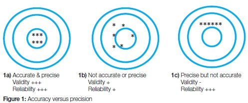
Results can have low accuracy but high precision and vice versa, which impact on the validity and reliability. An example to illustrate this would be aiming an arrow at the centre of a target. If all arrows are close together and in the centre of the target you have high accuracy and precision (Figure 1a). Results are then considered valid and reliable. If all arrows are both far away from the centre, and spread out, there is low accuracy, low precision. Results are neither valid nor reliable (Figure 1b). Lastly, if the arrows are all far off the centre but still all close to each other, it indicates that a mistake has been made, but the same mistake is made each time. Thus, there is low accuracy but high precision, and the results are not valid, despite being reliable (Figure 1c).^7,8

d) Validity refers to how appropriate and adequate the test is for that specific purpose. It also considers how correctly the results are interpreted and subsequently used.

 

 

A note on sensitivity and specificity.

Sensitivity and specificity are used as statistical measures to determine the effectiveness of a medical diagnostics. Sensitivity is a measure of the number of true positives and is calculated from the formula [true positive/true positive + false negative], while specificity is a measure of the amount of true negatives and is calculated by [true negative/true negative + false positive].

 

4. VARIABLE

This is the property of an object or event that can take on different values. For example, college major is a variable that takes on values like mathematics, computer science, English, psychology.¹

4.1 Discrete Variable has a limited number of values e.g. gender (male or female)

4.2 Continuous Variable can take on many different values anywhere between the lowest and highest points on the measurement scale.

4.3 Dependent Variable is that variable in which the researcher is interested, but is not under his/her control. It is observed and measured in response to the independent variable.

4.4 Independent Variable is a variable that is manipulated, measured, or selected by the researcher as an antecedent (precursor) condition to an observed behaviour. In a hypothesized cause-and-effect relationship, the independent variable is the cause and the dependent variable is the outcome or effect.

 

5. MEASURES OF CENTRE

Plotting data in a frequency distribution shows the general shape of the distribution and gives a general sense of how the numbers are bunched. Several statistics can be used to represent the "centre" of the distribution. These statistics are commonly referred to as measures of central tendency.¹

5.1 Mean (average) - is the most common measure of central tendency and refers to the average value of a group of numbers. Add up all the figures, divide by the number of values, and that is the average or mean It is calculated from the formula ΣΧ / N. [The sum all the scores in the distribution (ΣΧ) divided by the total number of scores (N)]. If you subtract each value in the distribution from the mean and then sum all of these deviation scores, the result will be zero (* see below). As one comic put it " Whenever I read statistical reports, I try to imagine the unfortunate Mr Average Person who has 0.66 children, 0.032 cars and 0.046 TVs".³

5.2 Median - is the score that divides the distribution into halves; half of the scores are above the median and half are below it when the data are arranged in numerical order. It is the central value, and can be useful if there is an extremely high or low value in a collection of values. The median is also referred to as the score at the 50^th percentile in the distribution. The median location of N numbers can be found by the formula (N + 1) / 2. When N is an odd number, the formula yields an integer that represents the value in a numerically ordered distribution corresponding to the median location. (For example, in the distribution of numbers (3 1 5 4 9 9 8) the median location is (7 + 1) / 2 = 4. When applied to the ordered distribution (1 3 4 5 8 9 9), the value 5 is the median, three scores are above 5 and three are below 5. If there were only 6 values (1 3 4 5 8 9), the median location is (6 + 1) / 2 = 3.5. In this case the median is half-way between the 3^rd and 4^th scores (4 and 5) or 4.5.

5.3 Mode - is the most frequent or common score in the distribution, and is the point or value of Χ that corresponds to the highest point on the distribution. If the highest frequency is shared by more than one value, the distribution is said to be multimodal, and will be reflected by peaks at two different points in the distribution.

 

6. MEASURES OF SPREAD

Although the average value gives information about how scores are centred in the distribution, the mean, median, and mode do not help much when interpreting those statistics. Measures of variability provide information about the degree to which individual scores are clustered about, or deviate from the average value in a distribution.¹

6.1 Range is the difference between the highest and lowest score in a distribution. It is not often used as the sole measure of variability because it is based solely on the most extreme scores in the distribution and does not reflect the pattern of variation within a distribution.

a) Interquartile Range (IQR) provides a measure of the spread of the middle 50% of the scores. The IQR is defined as the 75^th percentile - the 25^th percentile. The interquartile range plays an important role in the graphical method known as the boxplot. The advantage of using the IQR is that it is easy to compute and extreme scores in the distribution have much less impact. However, it suffers as a measure of variability because it discards too much data. Nevertheless, researchers want to study variability while eliminating scores that are likely to be accidents. The boxplot allows for this for this distinction and is an important tool for exploring data.

6.2 Variance is a measure based on the deviations of individual scores from the mean. As noted in the definition of the mean (5.1 above), simply summing the deviations will result in a value of 0. To get around this problem the variance is based on squared deviations of scores about the mean. When the deviations are squared, the rank order and relative distance of scores in the distribution is preserved while negative values are eliminated. Then to control for the number of subjects in the distribution, the sum of the squared deviations is divided by n (population) or by n - 1 (sample). The formula for variance is thus s² = Σ(χ - Χ)² /(n-1). The result is the average of the sum of the squared deviations and it is called the variance.

6.3 standard deviation provides insight into how much variation there is within a group of values. It measures the deviation (difference) from the group's mean (average). The standard deviation (s or σ) is the positive square root of the variance. The variance is a measure in squared units and has little meaning with respect to the data. Thus, the standard deviation is a measure of variability expressed in the same units as the data. The standard deviation is very much like a mean or an "average" of these deviations. In a normal (symmetric and mound-shaped) distribution, about two-thirds of the scores fall between +1 and -1 standard deviations from the mean and the standard deviation is approximately 1/4 of the range in small samples (N< 30) and 1/5 to 1/6 of the range in large samples (N> 100).

Standard deviation and variance are both measures of variability. The variance describes how much each value in the data set deviates from the mean (i.e. the spread of the responses), and is a squared value. The standard deviation also describes variability and is defined as the square root of the variance. This allows for a description of the variability in the same units as the data. A low SD will mean that the points of data are close to the mean, and a high SD indicates that the data is spread over a wide range of values. The SD is also used to describe the margin of error in the statistical analysis. This is usually twice the SD, typically described by the 95% confidence level. Confidence intervals consist of a range of values (interval) that act as good estimates of the unknown population parameter. After a sample is taken, the population parameter is either in the interval or not. The desired level of confidence is set by the researcher beforehand, for example 90%, 95%, 99%. If a corresponding hypothesis test is performed, the confidence level is the complement of the level of significance, i.e. a 95% confidence interval reflects a significance level of 0.05. Greater levels of variance yield larger confidence intervals, and hence less precise estimates of the parameter. Certain factors may affect the confidence interval size including size of sample, level of confidence, and population variability. A larger sample size normally will lead to a better estimate of the population parameter.

 

7. measures of shape

For distributions summarizing data from continuous measurement scales, statistics can be used to describe how the distribution rises and drops.¹

7.1 Symmetric refers to distributions that have the same shape on both sides of the centre are called symmetric. A symmetric distribution with only one peak is referred to as a normal distribution.

7.2 Skewness refers to the degree of asymmetry in a distribution. Asymmetry often reflects extreme scores in a distribution.

a) Positively skewed is when the distribution has a tail extending out to the right (larger numbers). In this case, the mean is greater than the median reflecting the fact that the mean is sensitive to each score in the distribution and is subject to large shifts when the sample is small and contains extreme scores.

b) Negatively skewed is when the distribution has an extended tail pointing to the left (smaller numbers) and reflects bunching of numbers in the upper part of the distribution with fewer scores at the lower end of the measurement scale.

7.3 Kurtosis has a specific mathematical definition, but generally, it refers to how scores are concentrated in the centre of the distribution, the upper and lower tails (ends), and the shoulders (between the centre and tails) of a distribution.⁶

 

8. the hypothesis

A hypothesis is an assumption about an unknown fact. Donald Rumsfeld may have been trying to explain this when he said "We know there are known knowns; these are things we know we know. We also know there are known unknowns; that is to say we know there are some things we do not know. But there are also unknown unknowns - the ones we don't know we don't know".⁵Most studies explore the relationship between two variables, for example, that prenatal exposure to pesticides is associated with lower birth weight. This is called the alternative hypothesis. The null hypothesis (Ho) is the opposite of the stated hypothesis (i.e. there is no relationship in the data, or the treatment did not have any effect). Well-designed studies seek to disprove the Ho, in this case, that prenatal pesticide exposure is not associated with lower birth weight.

Tests of the results determine the probability of seeing such results if the Ho were true. The p-value indicates how unlikely this would be, or helps determine the amount of evidence needed to demonstrate that the results more than likely did not occur by chance. It describes the probability of observing results if the null hypothesis is true. P value describes the statistical significance of the data, and is set at an arbitrary value. These are usually set with a cut-off point of 0.05 (5%) or 0.01 (1%). E.g. data with a p value of 0.01 means there is only a 1% chance of obtaining that same result if there was no real effect of the experiment (a 1% chance that the null hypothesis is true). If the Ho can be rejected, then the test will be statistically 'significant' NB. Significant is a statistical term and does not mean important!

 

9. correlation

This refers to the association between variables, particularly where they move together.

9.1 Positive correlation means that as one variable rises or falls, the other does as well (e.g. caloric intake and weight).

9.2 Negative correlation indicates that two variables move in opposite directions (e.g. vehicle speed and travel time).

9.3 Causation must not be confused with correlation. Causation is when a change in one variable alters another, but causation flows in only ONE direction. It is also known as cause and effect. E.g. Sunrise causes an increase in air temperature, in addition sunlight is positively correlated with increased temperature. However, the reverse is not true - increased temperature does not cause sunrise.

a) Regression analysis is a way to determine if there is or is not a correlation between two (or more) variables and how strong any correlation may be. It usually involves plotting data points on an X/Y axis, then looking for the average causal effect. This means looking at how the graph's dots are distributed and establishing a trend line. Again, correlation is not necessarily causation. While causation is sometimes easy to prove, frequently it can often be difficult because of confounding variables (unknown factors that affect the two variables being studied). Again, once causation has been established, the factor that drives change (in the above example, sunlight) is the independent variable. The variable that is driven is the dependent variable (see point 4 above).

 

CONCLUSIONS

Understanding commonly used statistical terms should help clinicians decipher and understand research data analysis, and equip them with the knowledge needed to analyze results more critically. Perhaps then, the old adage of "All readers can read, but not all who can read are readers" will no longer be true of those reading the SADJ.

 

References

1. University of Barotseland, Statistics - Introduction to Basic Concepts, in bobhall.tamu.edu/FiniteMath/Introduction.html. 2014.         [ Links ]

2. Schoeman, H. Biostatistics for the Health Sciences, University of Medunsa, Editor. 2003: South Africa. p. 78-91.         [ Links ]

3. Wikipedia. http://www.brainyquote.com/quotes/keywords/statistics.html 2015.         [ Links ]

4. Senn, D., Weems, RA., Manual of Forensic Odontology. 5th ed., ed. C. Press. 1997. Chapter 3.         [ Links ]

5. Light, R., Singer, JD., Willett, JB. You can't fix by analysis what you bungled by design. Course materials, quotes, in https://advanceddataanalytics.net/quotes/. 2014.         [ Links ]

6. Wikimedia. Statistical terms used in research studies; a primer for media. 2015: journalistresource.org/research/statistics-for-journalists.         [ Links ]

7. Green Thompson, L. Multiple choice exam setting workshop. 2015, accessed information:http:/download.usmle.org/iwtu- torial/intro.htm: Johannesburg.         [ Links ]

8. Green Thompson, L. Multiple choie question paper setting. 2015, Accessed at: http:/www.nbme.org/publications/item-writing-manual/html: Johannesburg.         [ Links ]

 

 

Correspondence:
Leanne M sykes
Department of Prosthodontics, University of Pretoria.
E-mail: leanne.sykes@up.ac.za