


Services on Demand
Journal

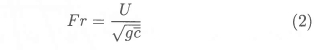
Article
 English (pdf)
 Article in xml format
 Article references
 Send this article by e-mail
Indicators
Related links
-
 Cited by Google
 -
 Similars in Google
Share

 Permalink
R&D Journal
On-line version ISSN 2309-8988Print version ISSN 0257-9669
R&D j. (Matieland, Online) vol.17 Stellenbosch, Cape Town 2001
Generalized vortex lattice method for prediction of hydrofoil characteristics
G.D. Thiart
Department of Mechanical Engineering, University of Stellenbosch, Stellenbosch, 7600 South Africa
ABSTRACT
The extension of the vortex lattice method for straight hydrofoils to hydrofoils of arbitrary shape is presented. The linearized free surface boundary condition and the radiation condition are satisfied by the vortex lattice, which is made up of "Kelvin" type bound vortex segments and semi-infinite trailing vortices parallel to the undisturbed free surface. Computational results are presented for the hydrodynamic characteristics (lift, wave plus induced drag) of a hydrofoil with a circular arc camber line, as function of Froude number, depth of submergence, aspect ratio, taper ratio, sweep angle, and dihedral angle.
Introduction
Knowledge of the forces and moments experienced by a hydrofoil of finite aspect ratio and arbitrary form in the proximity of a free surface is essential for the design of hydrofoil supported marine vehicles such as the HYSUCAT (HYdrofoil SUpported CATamaran) developed by Hoppe.1,2 Most of the methods known to this author for the computation of these forces and moments are based on lifting line theory (Kaplan & Breslin;3 Johnson;4 Furuya;5 Thiart6). Recently Thiart7 presented a vortex lattice method (VLM) for hydrofoils of rectangular planform which are essentially "flat", by which is meant that the foil has zero dihedral (but not necessarily zero camber). The extension of this VLM to hydrofoils of arbitrary form is presented in this paper, specifically for swept and tapered hydrofoils and hydrofoils with non-zero dihedral, as illustrated in Figure 1. Such hydrofoils have, for example, been found to provide "softer" riding HYSUCATs, in that the the foils exit and enter the water surface gradually rather than abruptly as is the case for rectangular flat foils.
The theory presented in the paper utilizes the same linearized free-surface boundary condition as for the flat rectangular hydrofoil, i.e.
Here the x-coordinate is defined as being in the direction of the onset flow (which has magnitude U), the z-coordinate is defined as being vertically upwards from the undisturbed free surface, u and w denote, respectively, the perturbation velocity components in the x- and z-directions, and k0= g/U2 is the wave number, with g the acceleration of gravity constant. The purpose of the theory is to compute the hydrodynamic characteristics of a hydrofoil in the form
where Cl and Cd denote, respectively, the coefficients of lift and of wave plus induced drag, CoP the position of the centre of pressure, α the geometrical angle of attack, Fr the Froude number, d the mean depth of submergence,  the mean chord length, Ar the aspect ratio, λ the taper ratio, Λ the sweep angle, and δthe dihedral angle of the hydrofoil. The usual definitions for the geometrical quantities α,
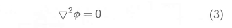
  , Ar, λ, Λ and δapply (see for example Bertin & Smith).8 The Froude number is based on the mean chord length, i.e.
Computational results are presented to illustrate the influence of the aspect ratio, taper ratio, sweep angle, dihedral angle, and effective angle of attack on the hydro-dynamic characteristics of a hydrofoil with a circular arc camber surface as function of Froude number and depth of submergence.
Theoretical model
Details of the conventional VLM, which applies to a hydrofoil in a fluid domain that extends to infinity in all directions, are well known (see for example Bertin & Smith).8 It is essentially a solution of Laplace's equation for a disturbance velocity potential Φ, i.e.
This disturbance potential has to fulfil the free surface boundary condition given by equation (1), the depth condition (∂Φ/∂z → 0 as z →∞), the flow tangency condition on the hydrofoil surface, and the radiation condition (free-surface waves generated by the disturbance may travel downstream only).
The disturbance is caused by the presence of a hydrofoil, and is superimposed on the uniform flow "seen" by the hydrofoil. The hydrofoil is usually thin, and is represented in the VLM by its camber surface (which has zero thickness). The camber surface itself is modelled by means of a vortex lattice, i.e. the camber surface is subdivided into a number of quadrilateral panels, for example as shown in Figure 1, and the influence of each one of these panels is represented by a so-called bound vortex located at is quarter-chord position. For the purposes of this paper it will be assumed that the hydrofoil is subdivided into M spanwise strips (extending from tip to tip) and N chord-wise strips (extending from the leading edge to the trailing edge), giving a total of MN panels. Also, following the findings of Hough,9 the lattice is inset one quarter of the spanwise vortex spacing from the tips of the hydrofoil.
According to the vortex laws of Helmholtz, the bound vortices cannot end in the fluid domain; they must form closed loops or extend to infinity. In the conventional VLM this is accomplished by trailing vortices that extend down-stream to infinity, usually in a direction parallel to the chord fine or mean camber surface of the hydrofoil. For the case under discussion, it is natural to have the trailing vortices extend downstream in a direction parallel to the undisturbed free surface. Furthermore, in the conventional VLM the trailing vortices are usually assumed to "leave" the camber surface directly at the endpoints of the bound vortices, thus forming not one but several "layers" of trailing vortices. For the case under discussion it is (intuitively) more correct to have a single layer of trailing vortices at a specific depth beneath the undisturbed free surface. To this end, for the purposes of this paper, the bound vortices are connected in a lattice structure that follows the curvature of the camber surface to the trailing edge, from where the trailing vortices extend downstream, as illustrated diagrammatically in Figure 2 for one half of a symmetrical hydrofoil. The relevant strengths of the bound vortices, "connecting" vortices and trailing vortices are indicated in Figure 3 for the nth chordwise strip of the lattice (the vortex strength on the ith spanwise and jthchordwise panel is indicated by Γi,j).
In the conventional VLM the components of the velocity induced at a general point (x,y,z) in the flow field are obtained by summing the influences of all the bound vortices, connecting vortices and trailing vortices. In order to satisfy also the linearized free surface boundary condition that is applicable here, it is necessary to add, for any one vortex segment, the influences of its image (in the undisturbed free surface) as well as its so-called wavemaking influences. Expressions for the computation of all these induced velocities are derived in the Appendix.
The strengths of the bound vortices are obtained, as for the conventional VLM, by application of the tangential flow boundary condition at the camber surface, in particular at control points located at the three-quarter chord position in the centre of each panel. In this way, a set of MN linear equations of the form
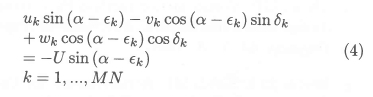
is established, wherein the MN Γs are the unknowns. In equation (4) uk, vk and wk represent the total contributions of all vortex segments to the components of induced velocity at the control point (xk,yk,zk), and εk and δk denote, respectively, the local camber angle and dihedral angle at the control point.
Once the system of equations represented by equation (4) has been solved, the lift and drag forces on the hydrofoil can be computed as in the conventional VLM, by means of the Kutta-Zhukovsky theorem. Thus, in dimensionless form,
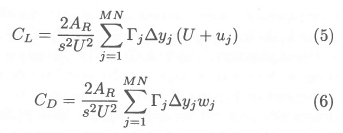
where ∆yjdenotes the "span width" of the chordwise strip on which panel j is located, and s the span width of the hydrofoil itself. The subscript j is used here instead of the subscript k in equation (4), to indicate that the velocities Uj and Wj have to be calculated at the centres of the relevant bound vortices - not at the control points. The leading edge moment can be computed in a similar way:
Computational results
All the results reported here were computed for a symmetrical hydrofoil with a 4.375% circular arc camber surface, at zero angle of attack (i.e. α = 0) and at a depth of sub-mergence equal to half a chord length. The zero-lift angle of attack for this camber surface is exactly -5°, according to thin airfoil theory; the effective angle of attack was therefore equal to 5° in all cases.
For every situation computations were performed on three progressively finer grids: 8 x 4, 16 x 8, and 32 x 16 panels on one half of the foil. The results were extrapolated to zero grid size using Richardson extrapolation. The order of extrapolation was estimated from the computational results on the three grids in the manner described by Ferzigier and Perić.12
Results for the lift are presented in terms of the ratio Cl/Cl∞,2D, where Cl is the computed lift coefficient and Cl∞,2D is the theoretical lift coefficient of the corresponding two-dimensional foil at infinite submergence (i.e. π2/18 here). Because drag is essentially proportional to the square of the lift, results for the drag (i.e. the "inviscid drag", which consists of the so-called vortex induced drag and the wave drag) are presented in terms of the ratio  , where Cd is the computed coefficient of drag. No results are presented for the centre-of-pressure, due to lack of space.
Results axe presented for Froude numbers from 0.5 to 20, although the range of practical interest is for Froude numbers higher than about 5. The discussion of the results that follow pertains to this range of interest.
Influence of aspect ratio:
Computations were carried out for zero-dihedral, rectangular hydrofoils with aspect ratios of 2, 5, 10 and ∞ (i.e. a two-dimensional hydrofoil). The variation of lift and drag as function of aspect ratio and Froude number are presented in Figures 4 and 5. It is clear that the lift is drastically reduced for small-aspect ratio hydrofoils; even more so than for hydrofoils at infinite submergence, where the theoretical reduction of lift for a wing with an aspect ratio of 5 would "only" be about 30%. The drag increases exponentially with decrease in aspect ratio.
Influence of taper ratio:
Computations were carried out for straight, zero-dihedral hydrofoils with taper ratios of 1,⅓, ¼, and 0, and an aspect ratio of 5. The variation of lift and drag as function of taper ratio and Froude number are presented in Figures 6 and 7. It is clear that lift and drag are not much affected for taper ratios between 1 and ¼, but that for a taper ratio of 0 (i.e. a doubly triangular hydrofoil) the lift is significantly reduced and the drag significantly increased. Surprisingly, a taper ratio of 1 (i.e. a rectangular hydrofoil) appears to be close to any optimum that may exist. This is contrary to the result for an infinitely submerged wing, where a taper ratio of about ⅓ is optimum.
Influence of sweep angle:
Computations were carried out for untapered, zero-dihedral hydrofoils with sweep angles of -30°, -15°, 0°, 15°, 30°, and 45°, and an aspect ratio of 5. The variation of lift and drag as function of sweep angle and Froude number are presented in Figures 8 and 9. It is clear that the lift is significantly reduced for sweep angles greater in absolute value than about 30°, whilst the drag appears to decrease almost linearly with sweep angle over the range for which the computations were performed.
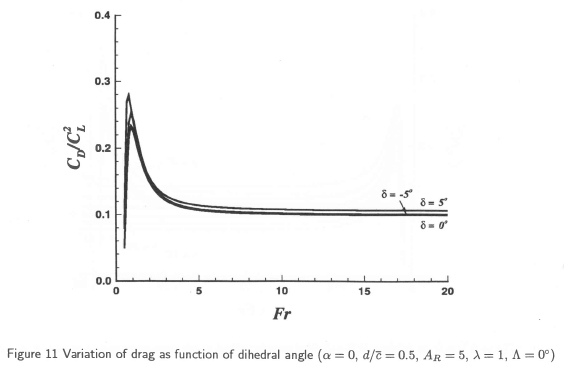
Influence of dihedral angle:
Computations were carried out for rectangular hydrofoils with di-hedral angles of -10°, -5°, 0°, and 5°, and an aspect ratio of 5. The variation of lift and drag as function of sweep angle and Froude number are presented in Figures 10 and 11. Neither the lift nor the drag seems to be significantly affected for these small dihedral angles, and it is apparent that a dihedral angle of 0° is close to any optimum that may exist.
Concluding remarks
From the computations presented in this paper, it can be concluded that the most efficient hydrofoil for steady motion is one with as large an aspect ratio as possible, no dihedral or taper, and swept back at an angle of approximately 30°.
The computations reported here are extremely CPU-intensive, even though the method is based on a linearized free-surface boundary condition. This is due mainly to the numerical integrations required for the computation of the induced velocities associated with the wave potential. Often not only lift, drag and centre-of-pressure results are required, but also the deformation of the free surface. The computation of the deformation of the free surface by means of the proposed method is certainly possible, but not really feasible as a very large number of points on the (infinite) free surface have to be computed. Therefore work is currently in progress to model the fully nonlinear free surface by means of a staggered grid higher order panel method similar to the one developed by Thiart and Bertram13 for the computation of flow over a two-dimensional hydrofoil. The results presented in this paper are proving to be of great value for comparative purposes.
References
1. Hoppe KGW. The HYSUCAT development. Ship Technology Research, 38, 134-139, 1991. [ Links ]
2. Hoppe KGW. Hydrofoil catamaran developments in South Africa. First International Conference on High-Performance Marine Vehicles, 1999, pp.92-101.
3. Kaplan P & Breslin JP. Evaluation of the theory for the flow pattern of a hydrofoil of finite span. Stevens Institute Technical Report No. 561, 1955.
4. Johnson RS. Prediction of lift and cavitation characteristics of hydrofoil-strut arrays. Marine Technology,2, 57-69, 1965. [ Links ]
5. Furaya O. Three-dimensional theory on supercavitating hydrofoils near a free surface. Journal of Fluid Mechanics, 71, 339-359, 1975. [ Links ]
6. Thiart GD. Numerical lifting fine theory for a hydrofoil near a free surface. R&D Journal, 10, 18-23, 1994. [ Links ]
7. Thiart GD. Vortex lattice method for a straight hydrofoil near a free surface. International Shipbuilding Progress, 44, 5-26, 1997. [ Links ]
8. Bertin JJ & Smith ML. Aerodynamics for Engineers. Prentice-Hall, Englewood Cliffs, New Jersey, 1979.
9. Hough GR. Remarks on vortex lattice methods. Journal of Aircraft, 10, 314-317, 1973. [ Links ]
10. Giesing JP & Smith AMO. Potential flow about two-dimensional hydrofoils. Journal of Fluid Mechanics,28, 113-129, 1967. [ Links ]
11. Hess JL & Smith AMO. Calculation of flow about arbitrary bodies. Progress in Aeronautical Sciences,8, 1-138, 1967. [ Links ]
12. Ferzigier JH & Perić M. Computational Methods for Fluid Mechanics. Springer, Berlin, 1996.
13. Thiart GD & Bertram V. Staggered grid panel method for hydrofoils with fully nonlinear free-surface effect. International Shipbuilding Progress,45, 313-329, 1998. [ Links ]
First received September 2000
Final version June 2001
Appendix
We consider the general vortex segment shown in Figure 12: it has strength Γand (vector) length 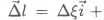
 Also shown in Figure 12 is an infinitesimal element on this vortex segment, located at position
 , with vector length
  . The velocity induced by this vortex element at the position
  can be obtained from the law of Biot-Savart, i.e.
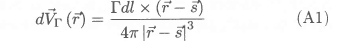
Upon substitution of the relevant quantities in equation (A1), the X-direction component of the induced velocity is obtained:
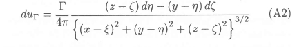
The X-direction component of the velocity induced at the position  by the image in the undisturbed free surface (i.e. the XY-plane) of the vortex segment is obtained in a similar manner:
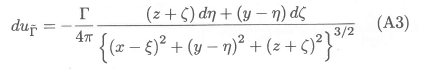
Specifically at z = 0, therefore the X-direction component of velocity induced by the vortex segment and its image is given by
This induced velocity will have a non-zero value only if the vortex segment is not parallel to the X-axis, i.e. if ∆η= ∆ζ = 0.
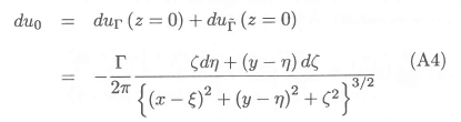
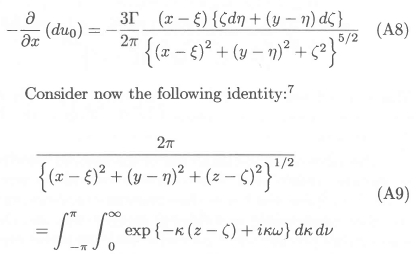
The value of the Z-component of the induced velocity at the free surface, dw0, is zero everywhere due to symmetry. The linearized free surface boundary condition can therefore be expressed as follows in terms of du0and the wavemaking potential dΦw associated with the vortex segment:
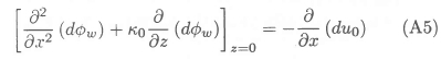
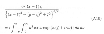
We consider first the left hand side of equation (A5). A useful solution of Laplace's equation, which also satisfies the depth condition, is7
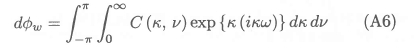
where ω = (x - ξ) cos v+(y - η) sin v, and C (k, v) a function that has to be determined, and where it is understood that only the real part is taken. We use this solution to obtain, for the left hand side of equation (A5),
Next we consider the right hand side of equation (A5). From equation (A4) we have
Taking derivatives with respect to x and z on both sides of equation (A9), yields the following result at z = 0:
Similarly, taking derivatives with respect to x and y on both sides of equation (A9), yields the following result at z = 0:

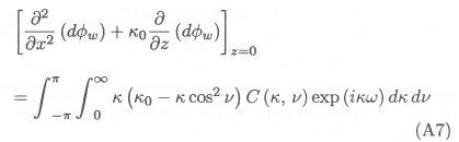
We now use equations (A8), (A10), and (All) to obtain, for the right hand side of equation (A5),
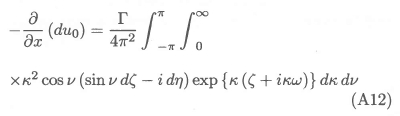
The function C (k, v) is obtained by substituting equations (A7) and (A12) into equation (A5):
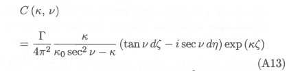
We denote by kv the term k0sec2v, and substitute equation (A13) into equation (A6) to obtain the velocity potential for the infinitesimal vortex element:
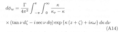
It can be shown, by using the periodic nature of the integrand with respect to v, that equation (A14) reduces to
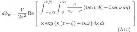
The integration with respect to k in equation (A15) can be performed utilizing the methodology of Giesing and Smith,10 whence it can be shown that it is necessary, in order to satisfy the radiation condition, to add the term
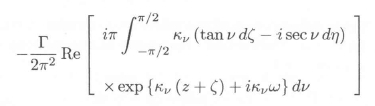
to the velocity potential. This term cancels out waves travelling upstream of the disturbance caused by the vortex segment. The velocity potential for the infinitesimal vortex segment is therefore
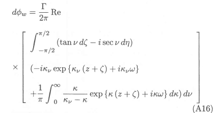
The wavemaking velocity potential of the whole vortex segment is obtained by integrating the expression for dΦw over the straight line connecting its "left hand" and "right hand" endpoints (ξl,ηl, ζl) and (ξr,ηr,ζr)- To this end we replace ξ by ξ0 + (∆ξ/∆η, where ξ0 = (ηrξl - ηlξr) /(ηr - ηl),and ζ by ζ0 + (∆ζ/∆η) η, where ζ0 = (ηrζl - ηlζr) / (ηr - ηl). The result of the subsequent integration with respect to η between ηl and ηr can be written in the following convenient format:
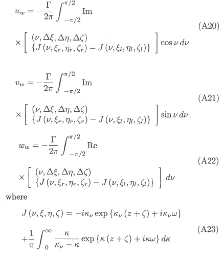
The components of the wavemaking velocity induced by the vortex segment are obtained in the usual manner by differentiation of Φw with to x, y, and z, respectively; the results can be written in the following convenient format:
Equation (A23) can be written as follows, by means of the methodology of Giesing and Smith:10
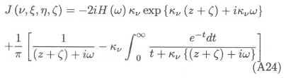
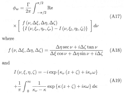
Here H(ω) denotes the Heaviside step function, which is equal to 1 if ω> 0 and equal to 0 otherwise. The remaining integral in equation (A24) can be evaluated numerically as described by Hess and Smith.11 The integration with respect to v in equations (A17) and (A20) to (A22) has to be done numerically; Gaussian quadrature is especially convenient in this respect, as it avoids the singularities at v = ±π/2 that are introduced by the function (v, ∆ξ, ∆η, ∆ζ) and the factor kv. Extensive numerical experimentation has shown that a reliable estimate for the required order NG of the Gaussian quadrature required for accurate results is the minimum of 1024 and the nearest integer to
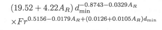
where dmin is the minimum depth of submergence of any point on the hydrofoil.
The "wavemaking" contribution  to the total velocity induced by the vortex segment is added to the contributions of the vortex segment itself and of its image in the undisturbed free surface,
  and
and  respectively.
The components of are obtained by integrating equation (A1) over the vortex segment; the result can be expressed as follows:
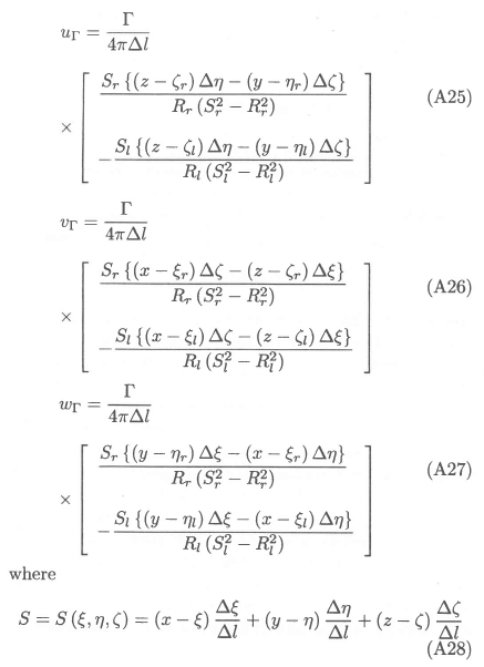
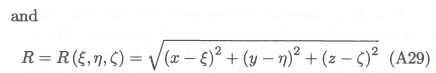
For the specific case of as trailing vortex extending to infinity in the X-direction, uΓ = 0, and equations (A27) and (A28) reduce to
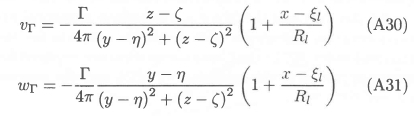
Expressions similar to equations (A25) - (A31) can be obtained for the components of  , by replacing in these equations Γby -Γ, ζz by ~ζz, ζr by -ζr, and Aζ by -Aζ. Hence it can be shown that
