


Services on Demand
Journal

Article
 English (pdf)
 Article in xml format
 Article references
 Send this article by e-mail
Indicators
Related links
-
 Cited by Google
 -
 Similars in Google
Share

 Permalink
Journal of the South African Institution of Civil Engineering
On-line version ISSN 2309-8775Print version ISSN 1021-2019
J. S. Afr. Inst. Civ. Eng. vol.57 n.3 Midrand Sep. 2015
https://doi.org/10.17159/2309-8775/2015/V57N3A2
TECHNICAL PAPER
Comparison of two data-driven modelling techniques for long-term streamflow prediction using limited datasets
O K Oyebode; J A Adeyemo; F A O Otieno
ABSTRACT
This paper presents an investigation into the efficacy of two data-driven modelling techniques in predicting streamflow response to local meteorological variables on a long-term basis and under limited availability of datasets. Genetic programming (GP), an evolutionary algorithm approach and differential evolution (DE)-trained artificial neural networks (ANNs) were applied for flow prediction in the upper uMkhomazi River, South Africa. Historical records of streamflow, rainfall and temperature for a 19-year period (1994-2012) were used for model design, and also in the selection of predictor variables into the input vector space of the model. In both approaches, individual monthly predictive models were developed for each month of the year using a one-year lead time. The performances of the predictive models were evaluated using three standard model evaluation criteria, namely mean absolute percentage error (MAPE), root mean-square error (RMSE) and coefficient of determination (R2). Results showed better predictive performance by the GP models (MAPE: 3.64%; RMSE: 0.52: R2: 0.99) during the validation phase when compared to the ANNs (MAPE: 93.99%; RMSE: 11.17; R2: 0.35). Generally, the GP models were found to be superior to the ANNs, as they showed better performance based on the three evaluation measures, and were found capable of giving a good representation of non-linear hydro-meteorological variations despite the use of minimal datasets.
Keywords: data-driven models, artificial neural networks, genetic programming, streamflow prediction, upper uMkhomazi River
INTRODUCTION
The need to manage water resources in arid and semi-arid regions has always been of high importance to water managers and decision-makers, especially in this era of increased climate variability. Water resources engineers and other stakeholders have developed various approaches to managing the relatively little amount of water in these regions in order to ensure constant availability of water for domestic, industrial, ecological and agricultural purposes. Streamflow remains a fundamental component of the water cycle and a major source of freshwater availability for human, animal, plant and natural ecosystems (Makkeasorn et al 2008). Therefore, prediction of streamflow both on a short-term and long-term basis is of crucial importance to water managers as it forms the basis upon which their decisions are made. While short-term predictions are made to provide signals about flood dangers and drought, long-term predictions help in providing information for long-term water supply strategies (Kisi & Cigizoglu 2007). Such information is needed, for example, when making decisions on the location and sizing of reservoirs on a river.
Numerous researchers have applied various approaches to predicting streamflow - from the use of traditional auto-regressive (AR) models (Jayawardena & Lai 1994; Wang et al 2009; Wu et al 2009), to the use of conceptual, process-based and physically-based models (also referred to as the "knowledge driven models") (Limbrick et al 2000; Butts et al 2004; Chiew 2006; Jiang et al 2007; Leander & Buishand 2007), to the data-driven models (DDMs) (Cannon & Whitfield 2002; Maity & Kashid 2010; Zakaria & Shabri 2012; Galelli & Castelletti 2013; Kasiviswanathan & Sudheer 2013). In recent years, the application of DDMs have gained more popularity due to their good performance when applied to complex hydrological modelling problems. DDMs are models that give representation of system state variables such as input, and internal and output variables, while characterising the nature of hydrological processes within the system. They do this by taking into account only a few assumptions about the physics of the system being modelled. DDMs are now being considered as an approach that could complement or replace the knowledge-driven models (Solomatine & Ostfeld 2008; Londhe & Charhate 2010). A major reason is that results from the latter have been found to exhibit higher-degree uncertainties in their structural makeup and parameterisations when compared to DDMs (Poulin et al 2011; Il-Won et al 2012; Montanari & Di Baldassarre 2013). Hence, the use of DDMs is seen as a promising technique for solving these sensitivity and uncertainty issues, as well as other hydrological modelling-related problems.
The genetic programming (GP) approach is a prominent DDM that has proven applicability to hydrological modelling. GP is a member of the evolutionary algorithm (EA) family and has been applied in a wide range of science-related and engineering analyses. GP has performed well in various water-related studies, such as sediment transport modelling, streamflow prediction, rainfall-runoff modelling, ecological modelling, uncertainty assessment studies, etc (Liong et al 2002; Muttil & Lee 2005; Ni et al 2010; Garg 2011; Selle & Muttil 2011; Sirdari et al 2011; Kisi et al 2012).
Another extensively used data-driven modelling technique is artificial neural networks (ANN). ANN is inspired by neuroscience and uses its adaptive learning feature to solve problems in domains with little or no prior knowledge of the system being modelled. Over the last two decades, ANN has been successfully applied to various fields of water resources, including function approximation, classification and forecasting studies (Coulibaly et al 2001; Moradkhani et al 2004; Cigizoglu 2005; Dibike & Coulibaly 2006; Kisi & Cigizoglu 2007; Heng & Suetsugi 2013). With the incorporation of ANNs, ensembles of models are being built to form modular or hybrid models in order to increase the confidence level of predictive assessment studies and to reduce model uncertainty (Abrahart et al 2012).
However, in order to achieve accurate and reliable predictions in hydrological studies, large datasets are often required for the purpose of model training (Babovic & Keijzer 2002). These huge numbers of datasets are limited to certain regions and are often unavailable in some areas, especially in developing countries (Ni et al 2012).
The main objective of this study is to develop models capable of long-term streamflow prediction in response to non linear fluctuations of meteorological variables in the upper uMkhomazi River. The potentials of the GP and ANN approach in providing models, using the few available datasets, were subjected to test and their performances evaluated comparatively so as to determine the suitable approach for streamflow prediction in the study area. This study is unique, as comparative studies between two evolutionary-inspired techniques (GP and a DE-trained ANN) are very uncommon, especially when employed under limited availability of datasets.
STUDY AREA AND DATASETS
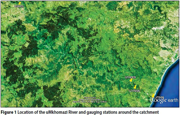
The upper uMkhomazi River is located within the province of KwaZulu-Natal in South Africa, and is the third largest river in the province. The river is of high importance due to its role as a major source of water supply to the densely populated urban areas of Durban and Pietermaritzburg. The uMkhomazi River is approximately 160 km long and is elevated at about 3 300 m above sea level. The river derives its source from the upper Drakensberg Mountains and discharges into the Indian Ocean, draining an area of 4 400 km2. The climate is characterised by wet summers which occur between November and March, and dry winters which extend over the months of June to September. Mean annual precipitation varies between 700 to 1 200 mm year-1, with highly intra- and inter-seasonal streamflows estimated to produce an average annual yield of 568 million m3 (Flugel & Marker 2003).
Past records of mean streamflow on a monthly basis were obtained from the Department of Water Affairs (DWA). Nineteen-year data from gauging station U1H005 (uMkhomazi River @ Lot 93 1821) with geographical coordinates between 29' 44' 37.3' south longitudes and 29' 54' 17.8' east latitudes were applied in this study (Figure 1). The South African Weather Service (SAWS) provided the corresponding climatic data from three independent weather data stations (Pietermaritzburg, Shaleburn and Giant's Castle) located within the study area.
METHODOLOGY
Genetic programming
Genetic programming (GP) (Koza 1992) is a population-based search which is inspired by the Darwinian principle of natural selection (survival of the fittest). GP is a member of the evolutionary algorithm (EA) family which performs its operations by genetically breeding a population of computer programs to solve problems. GP initialises by randomly generating programs that are perceived to be candidate solutions to the problem. Programs are then chosen from the pool, and evaluated based on a "fitness function" which describes how well they solve the given problem. The selected best programs are then transformed into a new generation of computer programs using genetic operators which apply slight modifications to the structure of the selected programs to achieve better solutions/programs. These successive iterations continue until a termination criterion is met. The program returned at the end of the run is finally chosen as the best program and the model that best solves the given problem. The principal operators employed in GP are:
1. Selection: Parent programs are chosen probabilistically based on their fitness values for the purpose of reproduction.
2. Crossover: A modification to the structure of the parent programs which involves swapping some sections to produce offspring programs.
3. Mutation: The creation of an offspring program by randomly altering a structural member or node of a selected parent program.
The GP representation consists of numerical constants and variables generally referred to as "terminals", T, and arithmetic, relational and trigonometric operations which are internal nodes called "functions" F. The selected terminals and functions constitute the primitive set of the GP algorithm. The five major preparatory steps that should be adopted before applying GP to a problem involve (i) selecting the set of terminals, (ii) selecting the set of primitive functions, (iii) determining the fitness function, (iv) determining the parameters for controlling the run, and (v) defining the criterion for terminating the run (Maity & Kashid 2009). The reader is referred to Koza (1992), Babovic & Keijzer (2000) and Poli et al (2008) for more in-depth discussion on GP.
Artificial neural networks (ANNs)
ANN is a computational intelligence (CI) method inspired by the neurological processing ability of the human brain. ANN models consist of a pool of simple processing units called neurons which communicate by sending signals to one another over a large number of weighted connections (Kröse & van der Smagt 1996). The operating principles of ANNs is based on parallel distributed information processing that is capable of storing experiential knowledge gained through the process of learning, and making it available for future use (Elshorbagy et al 2010). The processing units function by receiving inputs from external sources or other neurons in the network, and computing output signals which is transmitted to other units. These processing units are found in layers commonly categorised as input, hidden or output layers. The use of an activation function in the hidden node of ANNs helps in transforming the non-linearity in the inputs into a linear space. The commonly used activation functions are sigmoidal functions such as the logistic and hyperbolic tangent functions (Maier & Dandy 2000). The major network topologies that characterise the architecture of ANNs are the feed-forward neural networks (FFNN) and re-current neural networks (RNN); with multilayer perceptron (MLP), radial basis function (RBF) networks, Kohonen's self-organising feature maps (SOFM) and Elman-type RNN as the most popular ANNs (Coulibaly & Evora 2007; Jha 2007). Numerous specialised learning algorithms have been employed for the purpose of training and subjecting ANNs to adaptive learning. The earliest and most popular method that has been used to train ANNs is the back propagation (BP) algorithm. However, in recent times research has produced improved algorithms for ANN. These include methods based on gradient descent like quick propagation (QP) and the Levenberg-Marquardt (LM) algorithm, and heuristic methods such as genetic algorithm (GA) and differential evolution (DE). Hence, the ability of ANNs to assimilate complex and non-linear input-output interactions makes it suitable for predictive studies in the field of water resources.
Selection of input variables
The modelling strategy employed in this study was to subject the two approaches (GP and ANN) to the same set of datasets to avoid any form of bias. Hence, the same set of input variables were used for both models. However, the choice of input variables was dependent on the few available datasets. Although there are several processes that influence streamflow generation in river hydrology, such as precipitation, temperature, evaporation, soil moisture, vegetation cover, land use, etc (Loucks & van Beek 2005; Raghunath 2007), only the available datasets of rainfall and temperature were used alongside that of streamflow for input variable selection. The streamflow, rainfall and temperature data made available by the DWA and SAWS cover a 19-year period (1994-2012). The rainfall and temperature datasets were collected from three independent weather stations located within the study area. Results of serial correlation analysis show high correlation between the values of streamflow for the past three years and that of any pre-selected year. The results, however, revealed that streamflow for the pre-selected year had close relationship with rainfall and temperature values of the preceding year across the three independent weather stations. The datasets were split randomly into two subsets, with two thirds of the datasets used for model training and the remaining third for validation. The random splitting was done in a manner in which the validation datasets were within the range of the training datasets, thereby making the datasets representative of the same population.
MODEL DEVELOPMENT
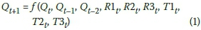
Both the GP and ANN models that were investigated for long-term streamflow prediction in this study were developed by adopting a monthly approach. It has been found that the use of individual monthly models in high-lead-time prediction produces better predictions when compared to the adoption of a single model, which often produces poor predictions (Sivapragasam et al 2011). Hence, a total of twelve individual monthly models (one for each month of the year) were developed using both modelling approaches. The input spaces of the GP and ANN models were populated with a total of nine input variables. These input variables comprised streamflow values for a given month in the last three years (Qt, Qt-1, Qt-2), rainfall values from the three independent weather stations for the same month in the preceding year (R1t, R2t, R3t) and their corresponding temperature values (T1t, T2t, T3t). Weather stations 1, 2 and 3 represent Pietermaritzburg (PMB), Shaleburn, and Giant's Castle weather stations respectively.
The approach employed for long-term streamflow prediction in this study was to adopt a one-year lead time. Therefore, the streamflow being modelled for a given month in the next year (Qt+1) is designated as the target output. The mathematical representation of the one-year lead time model adopted can be expressed as:
GP models
The GP predictive models for long-term streamflow prediction in this study were developed using an objective function - to minimise the mean-square error that can be obtained between the predicted and the observed values of streamflow. The mean-squared error function which measures the fitness of evolved programs is calculated by taking the average of the squared raw errors over the values in the training dataset. This can be expressed mathematically as:
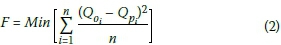
Qoand Qpare observed and predicted values of streamflow respectively, n is the number of data points, and i is the counter from 1 to the number of data points.
The ability of GP to screen and prioritise input variables during its run contributes to the fitness of the evolved programs, thus ensuring the accuracy of its predictions. This is achieved by expressing the contribution of each input variable as a function of its frequency of occurrence. The primitive set of the GP was supplied with arithmetic, comparison, logistic and trigonometric functions in order to capture details of the relationship between the input variables and the target output. A distributed population structure, which involves the subdivision of the population space into multiple subpopulation or demes, was employed in this study. This subdivision allows for occasional migration of individuals among demes for exchange of genetic material, in order to achieve evolution of the entire population, quicken the evolution process and also to prevent premature convergence.
The implementation of GP in this study was done by using a program-based GP tool called Discipulus (Francone 2011). Discipulus is a linear genetic programming (LGP) software that evolves models in the form of computer programs based on the least sum of squared errors. The goodness-of-fit is measured using R-square and F-score statistics against observed values of the training and validation datasets. The default parameter settings recommended by Francone (2011) were used to control the GP run (Table 1). Francone (2011) states that the default settings for a Discipulus project work quite well for most projects, and that Discipulus automatically sets, randomises, and optimises the GP parameters for project runs.

The GP algorithm for each computation was run on an Intel Core i7 PC with 3.40 GHz and 4 GB RAM. The maximum size of each evolved program was restricted to 512, initialising with 80 instructions per program. This was done to prevent the phenomenon of bloating, which means over-growing of programs without limits and without any improvement in the fitness of the population (Bleuler et al 2001).
ANN models
The multi-layer feed-forward neural network (FFNN), one of the most widely used network architecture in hydrological modelling systems, was employed for the purpose of comparison. The architectural design of the FFNN models developed comprise three layers - one input, one hidden and an output layer (Figure 2). The input layer consists of nine input nodes representing the nine selected input variables, while the output node consists of only one neuron (target output). The optimal architecture of each individual model was determined by incrementally varying the number of hidden layer nodes from 2 to 10 using a single (one) stepping approach.
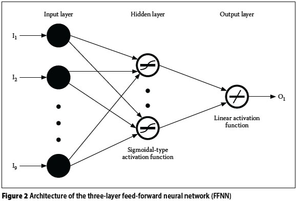
The ANN was trained using a differential evolution (DE) algorithm. A total run of 10 000 generations was adopted for optimal training after a number of trial runs. The population size, NP, crossover constant, CR, and mutation scale factor, F, were used to control amplification of differential variation during the run. Following the suggestion of Price and Storn (2013), NP, CR and F were set at "D multiplied by 10", 0.9 and 0.4 respectively, (where D is the number of weights and biases in the selected architecture). In the hidden layer of the FFNN, a logistic sigmoidal-type activation function of between 0 and 1 was used to scale the inputs in the range 0.1-0.9. A linear activation function was, however, employed in the output layer.
Performance evaluation
The performance of the models developed in this study was evaluated using three standard statistical measures, namely mean absolute percent error (MAPE), root mean-square error (RMSE) and coefficient of determination (R2). The three performance evaluation criteria can be computed using the following mathematical expressions: 1. The mean absolute percent error (MAPE): indicates a better model as its value approaches zero.

2. Root mean-square error (RMSE): indicates a better model as its value approaches zero.

3. Coefficient of determination (R2): indicates a better model as its value approaches 1.
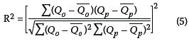
Qoand Qprepresent observed and predicted streamflows respectively, Qoand Qprepresent their corresponding mean values, n is the number of data points, and i is the counter from one to the number of data points. Considering that the maximum number of lags needed to predict the next year's flow is three, the 19-year datasets constituted 16 data points for each monthly model. Lower values of MAPE and RMSE would indicate better predictive accuracy of the model, while higher values of R2 (close to 1.0) would indicate better predictive accuracy of the models.
RESULTS AND DISCUSSIONS
The performance evaluation results of the two DDM approaches (GP and ANN) on long-term streamflow prediction in the upper uMkhomazi River are presented in Tables 2a and 2b, for the training and validation datasets respectively. It can be observed from Table 2a that both the GP and ANN models provided very competitive performances during the training phase, with the ANN models having a slight edge over the GP models. The maximum values of MAPE and RMSE recorded by the ANN models were 5.31% and 0.72 respectively, while their corresponding values in the GP models were computed to be 11.15% and 1.50. However, in both approaches, R-squared values showed a high correlation between observed and predicted streamflows. The R-squared values ranged between 0.9918-1.0000 in the ANN models, and 0.9891-0.9994 in the GP models.
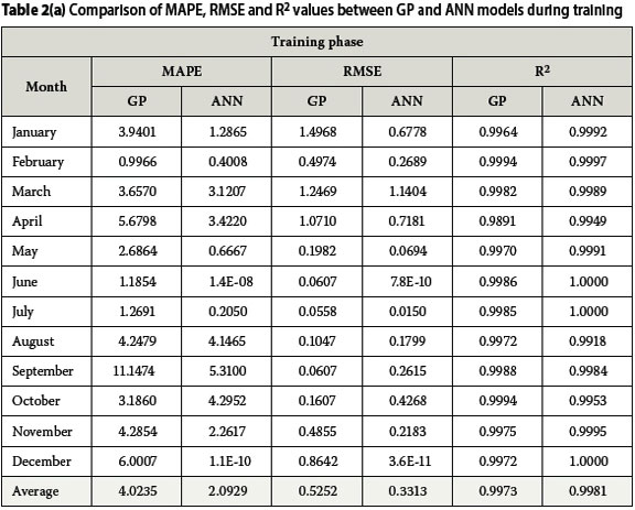
It can also be noted in both approaches that low flows, which occur during the months of May to July, produced smaller error estimates compared to the high flows which occur between December and March, with February as an exception.
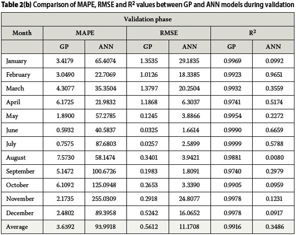
On the other hand, the GP models performed considerably better than the ANN models during validation, as the ANN models produced higher errors. The errors produced in the GP models during validation were better converged towards zero and are estimated to be 0.6%-7.6% and 0.03-1.38 for MAPE and RMSE respectively. Also, all the GP models maintained the highly positive correlations recorded during training, with R-squared estimates of 0.9740 -0.9999 during validation. It may be inferred that the ability of the GP approach to screen and prioritise input variables contributed to the fitness of its models (Makkeasorn et al 2008).
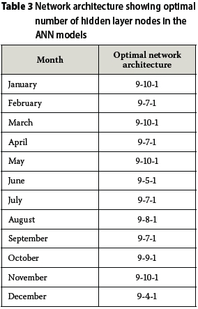
However, the error estimates in the DE-ANN models increased marginally, yielding higher MAPE and RMSE values while generating lower R-square values. Although the DE-ANN learning process was satisfactory, the generalisation was poor. The poor generalisation may be attributed to the use of small datasets (Zhang et al 2010), and also to the non-existence of an approach that could prevent over-training. Furthermore, it was noticed that the optimisation of the network architecture, as determined using the DE-algorithm, resulted in a slow convergence rate, and hence increased computational time. This can be understood better from Table 3, which presents the optimal network architecture of the individual ANN models as returned at the end of each run. It was observed during the runs that the training speed becomes slower as the number of hidden layer nodes increases. This implies that increase in the number of synaptic connections between units imposes a greater number of weights on the network. This is in line with the submission of Karthikeyan et al (2013) that the number of hidden layer nodes influence computational time, and consequently, that ANNs require an ample period of time for continuous training in order to achieve better convergence when used on small datasets. Some researchers (Ilonen et al 2003; Ghaffari et al 2006; Corzo & Solomatine 2007) have, however, opined that the idea of increasing the computational time should not be seen as a guarantee to achieving better generalisation, as this effort may yield no practical improvement in the results.
In contrast, GP exhibited better generalisation ability at a faster learning rate, a product of its ability to distribute the population into demes (Brameier & Banzhaf 2001). The distribution of the population into demes allowed for occasional migration of individuals between sub-populations for exchange of genetic materials, thereby leading to the occurrence of parallel evolution. This evolution further minimised the chances of the GP algorithm converging to local optima, and also ensured faster convergence.
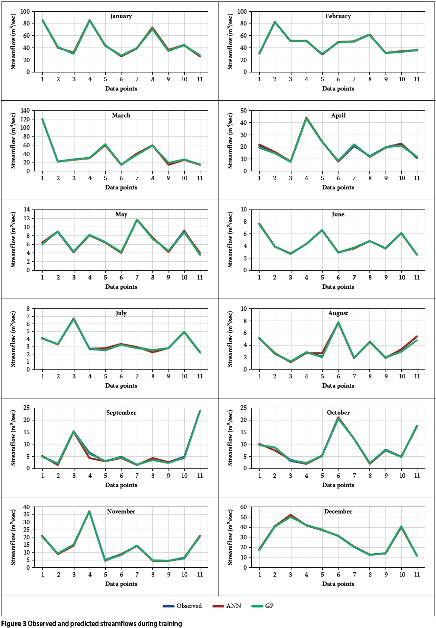
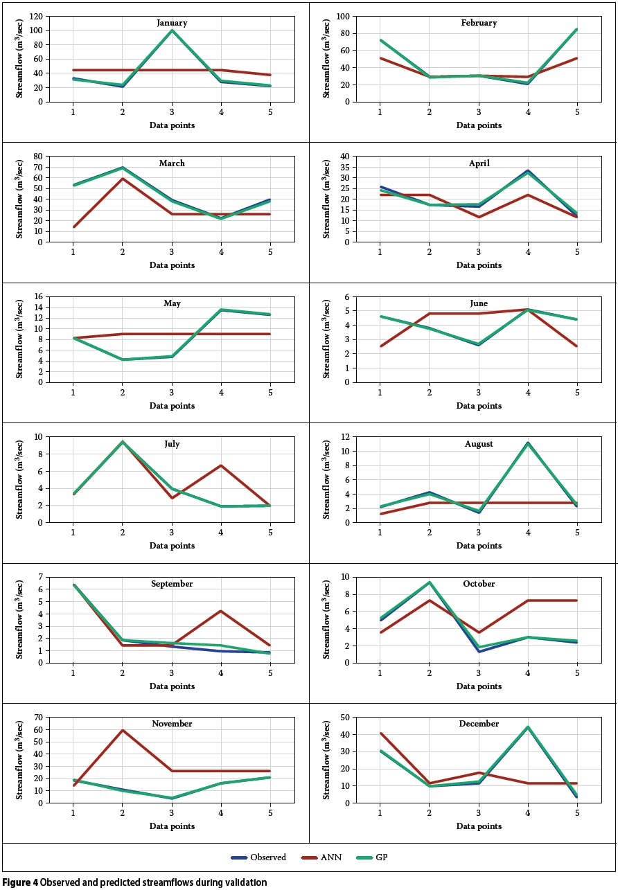
Figures 3 and 4 present plots of observed values against predicted values as simulated by the two approaches for both training and validation phases. The plots clearly reveal remarkable performance of the GP models during both training and validation, unlike the ANN models which were not able to replicate the performances recorded during the training phase, as a result of some under- or over-estimation of observed values. Despite ensuring that the validation datasets were within the range of the training datasets, the differences between observed and predicted streamflows during the months with high flows were more pronounced during validation.
The poor performance of the ANN models during validation is considered to be due to the problem of over-parameterisation and over-fitting, which is typical of ANNs (Bhattacharya et al 2001), especially when subjected to small numbers of datasets. This further indicates that the use of ANNs is problem-specific and data-dependent (Bhattacharya et al 2001), and that high difficulty exists in modelling hydrologic processes with limited datasets (Ni et al 2010).
On the contrary, the GP models in most cases simulated the streamflows closely and achieved better convergence than they did during training. Both the low and high flows were substantially reproduced by the GP models, including the spikes that characterised the streamflows in some months. This further affirms the ability of GP in capturing normal events, as pointed out in Londhe & Charhate's (2010) river flow predictive study. Also, the overfitting problems often associated with the ANNs were greatly minimised in the GP models, the reason being that GP ranks its potential candidate solutions (program models) in terms of their fitness, and often discard those with poor fitness. The ability of the Discipulus GP model to produce better solutions via the combination of the best single program models into team models (Francone 2011), also ensured the predictive accuracy of the GP models.
The consistency of the GP approach in simulating the hydro-climatological processes in the study area is evident, as the GP models were able to accurately capture the rainfall-temperature-streamflow relationship in each month of the year. The results agree with those in similar studies (Makkeasorn et al 2008; Guven 2009; Londhe & Charhate 2010), in which GP-derived models have also been found to showcase better predictive accuracy than the ANNs.
CONCLUSIONS
In this study, two data-driven modelling techniques, namely genetic programming (GP) and artificial neural networks (ANN), were employed comparatively for long-term streamflow prediction. Results clearly showed the efficacy of the GP approach in giving a better representation of complex and nonlinear input-output relationships, despite the use of limited datasets. The GP models developed obtained better performance as average values of mean absolute percent error (MAPE) = 4.02% and 3.64%; root mean-square error (RMSE) = 0.53 and 0.56, and R2 = 0.9973 and 0.9916 during training and validation respectively. However, the corresponding values ofMAPE, RMSE and R2 in the ANN models were estimated to be 2.09% and 93.99%; 0.33 and 11.17, and 0.9981 and 0.3486 respectively.
Though the use of ANNs remains a flexible approach known for its prominent feature of capturing non-linearity inherent in hydro-logical systems modelling, this study clearly showed that the large number of datasets required to achieve accurate and reliable results serve as a major drawback to its use, especially in areas where the availability of datasets is limited. Over-training could also have been a problem. The convergence rate of the DE-trained ANNs was found to be slower, requiring a considerable amount of time for model training. A potential solution in this regard is the hybridisation of learning algorithms, which is a combination of two or more learning algorithms for ANNs to achieve better adaptive learning.
In contrast to ANNs, the GP models trained faster and achieved better convergence, thereby producing close agreement between observed and predicted values, with highly positive correlations during both training and validation. Generally it can be concluded from this study that genetic programming can be employed for long-term streamflow prediction in the upper uMkhomazi River despite the limited availability of datasets. The monthly models developed can be deployed as predictive tools for the purpose of planning and management of water resources within the uMkhomazi region. In addition, this study further demonstrates GP as a powerful predictive tool in hydrologic modelling studies, which can be considered as an alternative approach to the ANNs, especially in data-sparse regions. Future work will focus on the conjunctive use of GP and other evolutionary computation techniques, such as screening and optimisation tools, for improving the performance of ANNs.
REFERENCES
Abrahart, R J, Anctil, F, Coulibaly, P, Dawson, C W, Mount, N J, See, L M, Shamseldin, A Y, Solomatine, D P, Toth, E & Wilby, R L 2012. Two decades of anarchy? Emerging themes and outstanding challenges for neural network river forecasting. Progress in Physical Geography, 36(4): 480-513. [ Links ]
Babovic, V & Keijzer, M 2000. Genetic programming as a model induction engine. Journal of Hydroinformatics, 2: 35-60. [ Links ]
Babovic, V & Keijzer, M 2002. Rainfall runoff modelling based on genetic programming. Nordic Hydrology, 33(5): 331-346. [ Links ]
Bhattacharya, M, Abraham, A & Nath, B. A 2001. Linear genetic programming approach for modeling electricity demand prediction in Victoria. Proceedings, Abraham, A & Koppen, M (Eds), International Workshop on Hybrid Intelligent Systems, 2001 Adelaide. Heidelberg: Physica-Verlag, pp 379-393. [ Links ]
Bleuler, S, Brack, M, Thiele, L & Zitzler, E 2001. Multiobjective genetic programming: Reducing bloat using SPEA2. Proceedings of IEEE Congress on Evolutionary Computation, Vol. 1: 536-543. [ Links ]
Brameier, M F & Banzhaf, W 2001. A comparison of linear genetic programming and neural networks in medical data mining. IEEE Transactions on Evolutionary Computation, 5(1): 17-26. [ Links ]
Butts, M B, Payne, J T, Kristensen, M & Madsen, H 2004. An evaluation of the impact of model structure on hydrological modelling uncertainty for streamflow simulation. Journal of Hydrology, 298(1): 242-266. [ Links ]
Cannon, A J & Whitfield, P H 2002. Downscaling recent streamflow conditions in British Columbia, Canada, using ensemble neural network models. Journal of Hydrology, 259(1): 136-151. [ Links ]
Chiew, F H 2006. Estimation of rainfall elasticity of streamflow in Australia. Hydrological Sciences Journal, 51(4): 613-625. [ Links ]
Cigizoglu, H K 2005. Application of generalized regression neural networks to intermittent flow forecasting and estimation. Journal of Hydrologic Engineering, 10(4): 336-341. [ Links ]
Corzo, G & Solomatine, D 2007. Baseflow separation techniques for modular artificial neural network modelling in flow forecasting. Hydrological Sciences Journal, 52(3): 491-507. [ Links ]
Coulibaly, P, Anctil, F & Bobee, B 2001. Multivariate reservoir inflow forecasting using temporal neural networks. Journal of Hydrologic Engineering, 6(5): 367-376. [ Links ]
Coulibaly, P & Evora, N 2007. Comparison of neural network methods for infilling missing daily weather records. Journal of Hydrology, 341(1): 27-41. [ Links ]
Dibike, Y B & Coulibaly, P 2006. Temporal neural networks for downscaling climate variability and extremes. Neural Networks, 19(2): 135-144. [ Links ]
Elshorbagy, A, Corzo, G, Srinivasulu, S & Solomatine, D 2010. Experimental investigation of the predictive capabilities of data-driven modeling techniques in hydrology. Part 1: Concepts and methodology. Hydrology and Earth System Sciences, 14(10): 1931-1941. [ Links ]
Flugel, W & Marker, M 2003. The response units concept and its application for the assessment of hydrologically related erosion processes in semiarid catchments of southern Africa. ASTM Special Technical Publication, 1420: 163-177. [ Links ]
Francone, F D 2011. Register Machine Learning Technologies, Inc. Discipulus Users Manual, Version 5. Available at: www.rmltech.com. [ Links ]
Galelli, S & Castelletti, A 2013. Assessing the predictive capability of randomized tree-based ensembles in streamflow modelling. Hydrology and Earth System Science Discussions, 10: 1617-1655. [ Links ]
Garg, V 2011. Modeling catchment sediment yield: A genetic programming approach. Natural Hazards: 70(1): 39-50. [ Links ]
Ghaffari, A, Abdollahi, H, Khoshayand, M, Bozchalooi, I S, Dadgar, A & Rafiee-Tehrani, M 2006. Performance comparison of neural network training algorithms in modeling of bimodal drug delivery. International Journal of Pharmaceutics, 327(1): 126-138. [ Links ]
Guven, A 2009. Linear genetic programming for time series modelling of daily flow rate. Journal of Earth System Science, 118(2): 137-146. [ Links ]
Heng, S & Suetsugi, T 2013. Using artificial neural network to estimate sediment load in ungauged catchments of the Tonle Sap River Basin, Cambodia. Journal of Water Resource and Protection, 5(2): 111-123. [ Links ]
Il-Won, J, Moradkhani, H & Chang, H 2012. Uncertainty assessment of climate change impacts for hydrologically distinct river basins. Journal of Hydrology, 466-467: 73-87. [ Links ]
Ilonen, J, Kamarainen, J-K & Lampinen, J 2003. Differential evolution training algorithm for feed forward neural networks. Neural Processing Letters, 17(1): 93-105. [ Links ]
Jayawardena, A & Lai, F 1994. Analysis and prediction of chaos in rainfall and stream flow time series.Journal of Hydrology, 153(1): 23-52. [ Links ]
Jha, G K. 2007. Artificial neural networks and its applications. Indian Agricultural Statistics Research Institute (IASRI), New Delhi. Available at: www.iasri.res.in/ebook/ebadat/5-Modeling%20and%20Forecasting%20Techniques%20in%20Agriculture/5-ANN_GKJHA_2007.pdf. [ Links ]
Jiang, T, Chen, Y D, Xu, C-Y, Chen, X, Chen, X & Singh, V P 2007. Comparison of hydrological impacts of climate change simulated by six hydrological models in the Dongjiang Basin, South China. Journal of Hydrology, 336(3): 316-333. [ Links ]
Karthikeyan, L, Kumar, D N, Graillot, D & Gaur, S 2013. Prediction of ground water levels in the uplands of a tropical coastal riparian wetland using artificial neural networks. Water Resources Management, 27(3): 871-883. [ Links ]
Kasiviswanathan, K & Sudheer, K 2013. Quantification of the predictive uncertainty of artificial neural network based river flow forecast models. Stochastic Environmental Research and Risk Assessment, 27(1): 137-146. [ Links ]
Kisi, O & Cigizoglu, H K 2007. Comparison of different ANN techniques in river flow prediction. Civil Engineering and Environmental Systems, 24(3): 211-231. [ Links ]
Kisi, O, Cimen, M & Shiri, J 2012. Suspended sediment modeling using genetic programming and soft computing techniques. Journal of Hydrology, 450-451: 48-58. [ Links ]
Koza, J R 1992. Genetic Programming: On the Programming of Computers by Means of Natural Selection. Cambridge, MA, US & London, UK: The MIT Press. [ Links ]
Kröse, B & Van Der Smagt, P 1996. An Introduction to Neural Networks. Amsterdam: University of Amsterdam. [ Links ]
Leander, R & Buishand, T A 2007. Resampling of regional climate model output for the simulation of extreme river flows. Journal of Hydrology, 332(3): 487-496. [ Links ]
Limbrick, K J, Whitehead, P, Butterfield, D & Reynard, N 2000. Assessing the potential impacts of various climate change scenarios on the hydrological regime of the River Kennet at Theale, Berkshire, south-central England, UK: An application and evaluation of the new semi-distributed model, INCA. Science of the Total Environment, 251: 539-555. [ Links ]
Liong, S Y, Gautam, T R, Khu, S T, Babovic, V, Keijzer, M & Muttil, N 2002. Genetic programming: A new paradigm in rainfall runoff modeling. Journal of the American Water Resources Association, 38(3): 705-718. [ Links ]
Londhe, S & Charhate, S 2010. Comparison of data-driven modelling techniques for river flow forecasting. Hydrological Sciences Journal, 55(7): 1163-1174. [ Links ]
Loucks, D & Van Beek, E 2005. Water Resources Systems Planning and Management: An Introduction to Methods, Models and Applications. Delft Hydraulics, the Netherlands: UNESCO Publishers. [ Links ]
Maier, H R & Dandy, G C 2000. Neural networks for the prediction and forecasting of water resources variables: A review of modelling issues and applications. Environmental Modelling & Software, 15(1): 101-124. [ Links ]
Maity, R & Kashid, S S 2009. Hydroclimatological approach for monthly streamflow prediction using genetic programming. ISH Journal of Hydraulic Engineering, 15(2): 89-107. [ Links ]
Maity, R & Kashid, S S 2010. Short-term basin-scale streamflow forecasting using large-scale coupled atmospheric-oceanic circulation and local outgoing longwave radiation. Journal of Hydrometeorology, 11(2): 370-387. [ Links ]
Makkeasorn, A, Chang, N B & Zhou, X 2008. Short term streamflow forecasting with global climate change implications - A comparative study between genetic programming and neural network models. Journal of Hydrology, 352(3-4): 336-354. [ Links ]
Montanari, A & Di Baldassarre, G 2013. Data errors and hydrological modelling: The role of model structure to propagate observation uncertainty. Advances in Water Resources, (51): 498-504. [ Links ]
Moradkhani, H, Hsu, K-L, Gupta, H V & Sorooshian, S 2004. Improved streamflow forecasting using self-organizing radial basis function artificial neural networks. Journal of Hydrology, 295(1): 246-262. [ Links ]
Muttil, N & Lee, J H W 2005. Genetic programming for analysis and real-time prediction of coastal algal blooms. Ecological Modelling, 189(3-4): 363-376. [ Links ]
Ni, Q, Wang, L, Ye, R, Yang, F & Sivakumar, M 2010. Evolutionary modeling for streamflow forecasting with minimal datasets: A case study in the West Malian River, China. Environmental Engineering Science, 27(5): 377-385. [ Links ]
Ni, Q, Wang, L, Zheng, B & Sivakumar, M 2012. Evolutionary algorithm for water storage forecasting response to climate change with small data sets: The Wolonghu Wetland, China. Environmental Engineering Science, 29(8): 814-820. [ Links ]
Poli, R, Langdon, W W B & McPhee, N F 2008. A Field Guide to Genetic Programming. London: Lulu Enterprises UK Limited. [ Links ]
Poulin, A, Brissette, F, Leconte, R, Arsenault, R & Malo, J-S 2011. Uncertainty of hydrological modelling in climate change impact studies in a Canadian, snow-dominated river basin. Journal of Hydrology, 409(3): 626-636. [ Links ]
Price, K & Storn, R. 2013. Differential evolution (DE) for continuous function approximation. Available at: www1.icsi.berkeley.edu/~storn/code.html [accessed on 19 July 2013]. [ Links ]
Raghunath, H M 2007. Hydrology: Principles, Analysis and Design. New Delhi: New Age International (Pvt) Ltd. [ Links ]
Selle, B & Muttil, N 2011. Testing the structure of a hydrological model using genetic programming. Journal of Hydrology, 397(1): 1-9. [ Links ]
Sirdari, Z Z, Ghani, A A & Hasan, Z A 2011. Prediction of bed load transport in Kurau River based on genetic programming. Paper presented at the 3rd International Conference on Managing Rivers in the 21st century: Sustainable Solutions for Global Crisis of Flooding, Pollution and Water Scarcity, 6-9 December 2011, Penang, Malaysia. [ Links ]
Sivapragasam, C, Muttil, N & Arun, V. Long-term flow forecasting for water resources planning in a river basin. Proceedings, International Congress on Modelling and Simulation, 12-16 December 2011, Perth, Australia, pp 4078-4084. [ Links ]
Solomatine, D & Ostfeld, A 2008. Data-driven modelling: Some past experiences and new approaches. Journal of Hydroinformatics, 10(1): 3-22. [ Links ]
Wang, W-C, Chau, K-W, Cheng, C-T & Qiu, L 2009. A comparison of performance of several artificial intelligence methods for forecasting monthly discharge time series. Journal of Hydrology, 374(3): 294-306. [ Links ]
Wu, C, Chau, K & Li, Y 2009. Predicting monthly streamflow using data-driven models coupled with data-preprocessing techniques. Water Resources Research, 45(8): W08432. [ Links ]
Zakaria, Z A & Shabri, A 2012. Streamflow forecasting at ungauged sites using support vector machines. Applied Mathematical Sciences, 6(60): 3003-3014. [ Links ]
Zhang, L, Merényi, E, Grundy, W M & Young, E F 2010. Inference of surface parameters from near-infrared spectra of crystalline H2OH2O ice with neural learning. Publications of the Astronomical Society of the Pacific, 122(893): 839-852. [ Links ]
 Correspondence:
Oluwaseun Oyebode
Department of Civil Engineering and Surveying
Durban University of Technology
PO Box 1334, Durban 4000
South Africa
T: +27 (0)84 807 3576
E: oluwaseun.oyebode@gmail.com
Dr Josiah Adeyemo
Prof Fred Otieno
Department of Civil Engineering and Surveying
Durban University of Technology
PO Box 1334, Durban 4000
South Africa
T: +27 (0)31 313 2985
E: josiaha@dut.ac.za
Prof Fred Otieno
Department of Civil Engineering and Surveying
Durban University of Technology
PO Box 1334, Durban 4000
South Africa
T: +27 (0)31 373 2375
E: otienofao@dut.ac.za

OLUWASEUN OYEBODE (MWISA, MIWA, MIAHS) is a Master's (research) candidate in Civil Engineering at the Durban University of Technology. He graduated with a BSc Upper Second Class Honours in Environmental Engineering from the University of Ibadan, Nigeria. His focus is in the fields of hydrological modelling and climate change impacts on water resources, with particular interest in the development of models using evolutionary computation and artificial intelligence techniques. His current research relates to the use of genetic programming and differential evolution-trained neural networks to model streamflow response to local hydro-climatic variables in the upper uMkhomazi River.

DR JOSIAH ADEYEMO (MASABE, MASCE, MIWA, MWISA) is a Senior Lecturer in the Department of Civil Engineering and Surveying at the Durban University of Technology. He obtained his BSc (Honours) at the University of Ilorin, Nigeria, his MSc at the University of Ibadan, Nigeria, and his doctorate at the Tshwane University of Technology. He focuses on developing and applying evolutionary optimisation techniques to solve real-world science and engineering design problems at minimum cost and for maximum benefit. He is renowned for the development of a multi-objective evolutionary algorithm called multi-objective differential evolution algorithm (MDEA) which is used by many researchers worldwide.

PROF FRED OTIENO Pr Eng (FSAICE, SFWISA) is a C-rated researcher with the National Research Foundation (NRF), South Africa. He is a Fellow of the South African Institution of Civil Engineering, a Senior Fellow of the Water Institute of Southern Africa (WISA), and was the WISA President in 2007/2008. He has over 30 active years of consulting, lecturing and research experience in a number of disciplines, more recently focusing on water resources management, water and wastewater treatment, solid waste management and general environmental management.
