TECHNICAL NOTE

 

Creating a conceptual hydrological soil response map for the Stevenson Hamilton Research Supersite, Kruger National Park, South Africa

 

 

George van Zijl; Pieter Le Roux

Department of Soil, Crop and Climate, University of the Free State, Bloemfontein, 9301, South Africa

Correspondence

 

 

---

ABSTRACT

The soil water regime is a defining ecosystem service, directly influencing vegetation and animal distribution. Therefore the understanding of hydrological processes is a vital building block in managing natural ecosystems. Soils contain morphological indicators of the water flow paths and rates in the soil profile, which are expressed as 'conceptual hydrological soil responses' (CHSR's). CHSR's can greatly aid in the understanding of hydrology within a landscape and catchment. Therefore a soil map could improve hydrological assessments by providing both the position and area of CHSR's. Conventional soil mapping is a tedious process, which limits the application of soil maps in hydrological studies. The use of a digital soil mapping (DSM) approach to soil mapping can speed up the mapping process and thereby extend soil map use in the field of hydrology. This research uses an expert-knowledge DSM approach to create a soil map for Stevenson Hamilton Research Supersite within the Kruger National Park, South Africa. One hundred and thirteen soil observations were made in the 4 001 ha area. Fifty-four of these observations were pre-determined by smart sampling and conditioned Latin hypercube sampling. These observations were used to determine soil distribution rules, from which the soil map was created in SoLIM. The map was validated by the remaining 59 observations. The soil map achieved an overall accuracy of 73%. The soil map units were converted to conceptual hydrological soil response units (CHSRUs), providing the size and position of the CHSRUs. Such input could potentially be used in hydrological modelling of the site.

Keywords: Digital soil mapping, terrain analysis, ecosystem services, conceptual hydrological soil responses, SoLIM

---

 

 

INTRODUCTION

Water is probably the defining element in all natural ecosystems. Hydrological processes determine the amount, seasonality and location of water, therefore rendering ecological system services, by directly influencing soils, wetlands and rivers controlling vegetation and animal distribution. The importance of a clear understanding of the hydrological processes in the management of water resources is augmented in the highly variable hydrological environment of southern Africa (Wenninger et al., 2008). The identification, definition and quantification of the flowpaths and residence times of the different components of flow are central to the understanding of hydrological processes. There exists an interactive relationship between soil and hydrology. As soil formation is influenced by climate, vegetation/land use, topography, parent material and time (Jenny, 1941), soil properties incorporate the influence of these factors in hydrologic flow paths. Therefore soil can be a first-order control in partitioning hydrological flow paths, residence times and distributions and water storage (Soulsby et al., 2006). Thus soil properties contain unique signatures of the hydrological regime under which they formed. Concepts developed about the soil water regime by field observations and quantification (Van Tol et al., 2011) make it possible to predict the conceptual response of different soil forms (Ticehurst et al., 2007; Van Tol et al., 2010; Kuenene et al., 2011). A soil map can be the basis to provide both the size and position of conceptual hydrological soil responses (CHSR's). This information could potentially improve hydrological parameterisation for predictions in ungauged basins.

Unfortunately, conventional methods of soil mapping are time consuming and expensive, limiting the application thereof in hydrology. However, based on the rapid improvement in information technology, remote sensing, digital elevation models (DEM's), pedometrics and geostatistics, digital soil mapping (DSM) methods are available which reduce the cost and time needed for soil surveying (Hensley et al., 2007). In South Africa, such methods have rarely been applied, and there remains a large scope for DSM research in local geographical settings and application to local needs.

In the Kruger National Park the so-called 'Supersites' project (Smit et al., 2013) has been launched to combine the research done in many disciplines within the Park on specific representative sites. Four sites were chosen to represent the main climatic and ecological regions within the Park. This project is part of a baseline study on the hydrology of the Stevenson Hamilton Research Supersite. This paper explains how a DSM exercise was done to create a CHSRU map for the Supersite. The hypothesis expressed is that DSM could provide the input to determine the position and area of the CHSRs, creating conceptual hydrological soil response units (CHSRUs) cost effectively and within acceptable time limits.

 

SITE DESCRIPTION

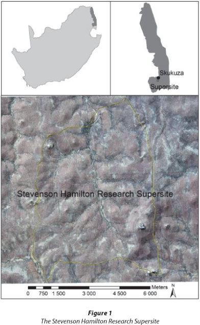
The study site is the 4 001 ha Stevenson Hamilton Research Supersite, approximately 7 km south of Skukuza in the Kruger National Park (Fig. 1). The mean annual precipitation is 560 mm/a (Smit et al., 2013), and the geological formation is granite and gneiss of the Nelspruit Suite (Venter, 1990). It lies in the Renosterkoppies land type (Venter, 1990). Furthermore it is a highly dissected landscape, with a high stream density (Smit et al., 2013), and a few prominent inselbergs occurring as rock outcrops. Combretum apiculatum and Combretum zey-heri dominate the woody vegetation on the crests. A distinct seepline commonly occurs between the crest and the mid-slopes, where Terminalia sericea is noticeable. Acacia nilotica and other fine-leaved woody species are most abundant on the midslopes and footslopes. Sodic sites frequently occur, commonly associated with Eucleadi vinoriumis (Smit et al., 2013). There is a very good correlation between the vegetation and soil type (Venter, 1990).

 

 

MATERIALS AND METHODS

Data acquisition

A suite of environmental covariates were assembled including Spot 5 (SPOT image, 2013), Landsat (USGS, 2013) satellite images, remotely-sensed biomass and evapotranspiration (ET) for a series of dates (eLeaf, 2013) and the SUDEM (Van Niekerk, 2012) digital elevation model (DEM). The SUDEM was re-interpolated to a 10 m and 30 m resolution, as multi-resolution elevation layers are useful to highlight different soil-terrain interactions. Topographic variables were derived from both DEMs with the basic terrain analysis tool in SAGA (SAGA User Group Association, 2011). Several additional co-variate layers, such as NDVI, were created by mathematical manipulation of the different bands of the Landsat and SPOT 5 images.

Field sampling

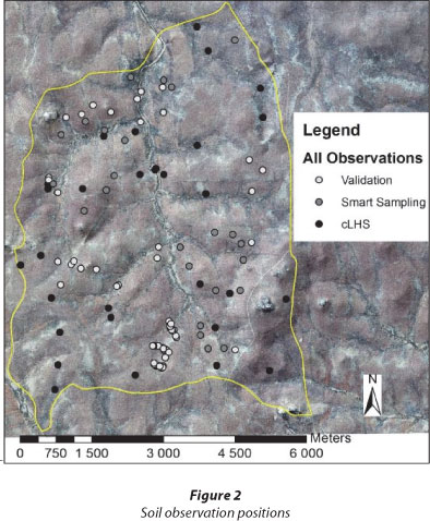
Three different sampling strategies were followed. For the training observations, both 'smart sampling' and conditioned Latin hypercube sampling (cLHS) (Minasny and McBratney, 2006) were used. For the smart sampling a colour aerial photograph was subjectively divided into 5 classes, and observation positions were chosen to include all 5 of the classes. Twenty-five smart sampling observations were made. Six co-variate layers were included into the cLHS. These layers were the principal component analysis (PCA) results of the ET, biomass, Landsat images, SPOT 5 images and both resolutions' topographic variable layers. Thirty observation positions were selected, of which one was rejected due to being too close to a road. Thus 29 observations were made by cLHS. Fifty-nine validation observations were at in-field determined positions, with soil surveyors walking transects through the study site, visually selecting representative sites where observations could be made. In this way, the entire study site was covered. The smart sampling and cLHS ensured that the whole attribute space was sampled, whereas the in-field determined sampling ensured full spatial coverage (Fig. 2). Soil observations were classified according to the South African soil classification system (Soil Classification Working Group, 1991). Hand-estimated texture, structure, mottles and stoniness were also observed per soil horizon.

 

 

Soil map creation

The soil observations were divided into 7 soil map units (SMUs) based on texture and the occurrence of a horizon with redox morphology. Descriptions of the SMUs are shown in Table 1. The SMUs were mapped by creating soil-landscape rules for each in SoLIM (Zhu, 1997). Central to these rules is an understanding of the soil distribution, based on the expert knowledge gained during field work for both the training and validation observations. Specific values for the rules are obtained from the values for the different covariates of the training soil observations only. The rules were derived by starting with the easiest, accurately identifiable SMU, the Sodic Soils. Once this SMU was mapped satisfactorily, the rules which defined its distribution were inverted for the other SMUs. Then the Clayey Soils were separated from the Sandy Soils. Lastly, within both the Clayey and Sandy Soils the soils with redox morphology within the profile were distinguished from the soils without redox morphology within the profile.

By running an inference of the soil map rules, SoLIM created a soil map for the area. The raster layer soil map was converted to a shapefile, and filtered using a majority filter with a square radius of 2 pixels and a 20% threshold. Polygons smaller than 4 pixels were manually included into larger, surrounding polygons. Alluvial soils were mapped by setting buffers around the channel network, which was delineated from the DEM in SAGA. The distance of the buffers were determined by the observations of how far alluvial soils occurred around the different stream orders. Rock outcrops were mapped manually from an aerial photograph, following the effort principle, i.e., that, if possible and more efficient, it is better to map areas than to predict them (McBratney et al., 2002).

The map was validated using the independent validation observations. Map accuracy was calculated as a percentage of correctly predicted point observations. A 1-pixel buffer was included around SMUs, as in Van Zijl et al. (2012). An accuracy matrix was created to evaluate the accuracy of each SMU.

Conversion from soil map to hydrological soil map

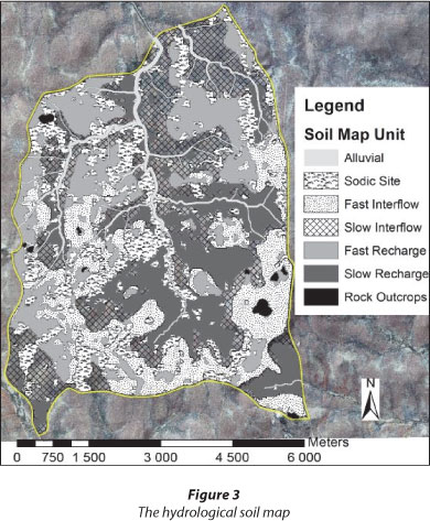
To create a hydrological soil map, a CHSR was assigned to each SMU according to Van Tol et al. (2013). Thus the hydrological soil map is a spatial representation of the CHSR of the study area, based on the distribution of the SMUs. Recharge soils are defined as soils where the dominant water flow path is one where the free water leaves the evapotranspiration zone, and recharges the lower vadoze zone. Interflow soils are soils where the dominant flow path is where free water flows laterally within the upper and intermediate vadoze zone, while responsive soils refer to soils where the dominant flow path is overland flow, due to either shallow soils with limited storage capacity or soils saturated with water for long periods (Van Tol et al., 2013).

 

RESULTS AND DISCUSSION

The observation positions give a good spatial coverage of the study area. The clusters that formed are due to the in-field determined sampling. The total of 113 observations is very little compared to the 2 000 which would have been necessary to draw a soil map of a 150 m grid with conventional methods. Thus a considerable cost and time saving was made.

The SMUs were grouped on the basis of hydrological response (Van Tol et al., 2013). This also meant that observations of the same soil form could be included into different CHSRUs, such as the Bonheim soil form which fits into both the Clayey Interflow and Clayey Recharge classes. The division was made on the basis of whether or not the C-horizon displayed signs of redox morphology. The Oakleaf and Tukulu soil forms also fit into two CHSRUs. Only when it was clear that the soil had formed due to alluvial deposits, was it added to the Alluvial SMU; otherwise the observation was added to the Sandy Interflow or Sandy Recharge SMU. The distinct seepline where Terminalia sericea is noticeable commonly occurs above the Sodic Site SMU. Here the Glenrosa soil form (Leptosols) is dominant. It was not mapped as it is too thin to be discernable at a 30 m resolution.

The SoLIM rules for the five SMUs mapped with SoLIM are shown in Table 2. Both topographic and vegetation indicating covariates were used, indicating that of the five soil-forming factors, not one dominates soil formation in this area. Vegetation is determined by the soil type, rather than playing a big role in the soil formation in this area. However, the parent material plays a dominant role in soil formation. The main geological formation of the area is granite, which weathers to a coarse sandy material, except in extreme cases where Sodic Sites develop. It is however highly unlikely for soils with melanic A horizons (Bonheim, Milkwood, Mayo) to occur. These soils are associated with basic intrusive rocks (Le Roux et al., 2013). Unfortunately the scale of the geological map did not allow for dolerite dykes (which are known to occur in the area) to be mapped. The soil map (Fig. 3) shows that there are considerable areas of Clayey Recharge and Clayey Interflow soils, which are largely comprised of soil forms with melanic A horizons. Thus the soil map could be improved if the location and extent of the influence of the dolerite dykes could be mapped.

 

 

 

 

The overall soil map accuracy of 73% (Table 3) is acceptable. This is higher than the 65% commonly accepted as the map accuracy of conventional soil maps (Marsman and De Gruijter, 1986). It also compares well with other studies using comparable methodology, such as the 69% of MacMillan et al. (2010), 69% of Van Zijl et al. (2012), and 76% of Zhu et al. (2008).

 

 

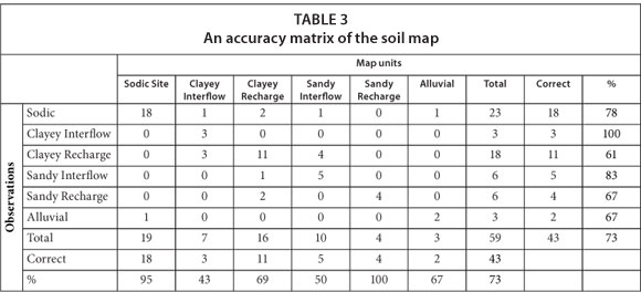
A concern though is the low accuracy values for the Clayey Interflow and Sandy Interflow map units. Seven of the soil observations made on the areas of these map units are actually Clayey Recharge soil observations. Thus the Clayey Interflow and Sandy Interflow SMUs are too large and the Clayey Recharge SMU is too small. To improve the map, the rules predicting the boundaries of these three SMUs need to be improved by observations made along the SMU boundaries. In contrast to this, with conventional methods a whole new survey would have to be done in order to improve the existing map.

The CHSRU map (Fig. 4) shows that 41% of the study area is covered by Interflow soils, 40% by Recharge soils and 19% by Responsive soils. However the great advantage of the mapping approach to determining those values is that the position of these soils is also known. This could be invaluable information to hydrological modellers; however, ways to exploit such input should be developed.

 

 

CONCLUSIONS

It was shown that a DSM approach could provide both the size and position of CHSRUs for a large area in a time-and cost-effective way. One hundred and thirteen (113) soil observations were made to create a soil map which is 73% accurate. In contrast to this, 2 000 soil observations would have been necessary in conventional soil mapping. The map could be improved with a geological map showing the dolerite dykes, as well as by making more observations on the boundaries between the Sandy Interflow, Clayey Interflow and Clayey Recharge SMUs, as pointed out by the error matrix. For this improvement only observations along the SMU boundaries of the three SMUs in question is necessary, in contrast to a new survey which would be required when using conventional methods.

The size and position of the CHSRUs could possibly be useful in improving predictions in ungauged basins, but methodology should be developed to accommodate such input into models. The first step may be to develop conceptual hydrologi-cal response models for hillslopes/soilscapes.

 

ACKNOWLEDGEMENTS

We would like to acknowledge the South African National Space Agency for providing the SPOT 5 and Landsat images, and the Department of Geography, Stellenbosch University, for providing us with the SUDEM. Furthermore we would like to thank the Water Research Commission and the University of the Free State for financial assistance.

 

REFERENCES

eLEAF (2013) Data supplied by the the Inkomati Catchment Management Agency on behalf of eLeaf (www.eleaf.com) and the WATPLAN EU project.         [ Links ]

HENSLEY M, LE ROUX PAL, GUTTER J and ZERIZGHY MG (2007) Improved soil survey technique for delineating land suitable for rainwater harvesting. WRC Report No. K8/685/4. Water Research Commission, Pretoria.         [ Links ]

JENNY H (1941) Factors of Soil Formation, a System of Quantitative Pedology. McGraw-Hill, New York.         [ Links ]

KUENENE BT, VAN HUYSSTEEN CW, LE ROUX PAL and HENSLEY M (2011) Facilitating interpretation of the Cathedral Peak VI catchment hydrograph using soil drainage curves. S. Afr. J. Geol. 114 525-234.         [ Links ]

LE ROUX PAL, DU PLESSIS MJ, TURNER DP, VAN DER WAALS J and BOOYENS HB (2013) Field Book for the Classification of South African Soils. South African Soil Surveyors Organization, Bloemfontein. 173 pp.         [ Links ]

MACMILLAN RA, MOON DE, COUPE RA, and PHILLIPS N (2010) Predictive ecosystem mapping (PEM) for 8.2 million ha of forest-land, British Columbia, Canada. In: Boettinger JL, Howell DW, Moore AC, Hartemink AE and Kienast-Brown S (eds.) Digital Soil Mapping; Bridging Research, Environmental Application and Operation. Springer, Dordrecht.         [ Links ]

MARSMAN BA, and DE GRUIJTER JJ (1986) Quality of soil maps, a comparison of soil survey methods in a study area. Soil Survey papers no. 15. Netherlands Soil Survey Institute, Stiboka, Wageningen.         [ Links ]

McBRATNEY AB, MINASNY B, CATTLE SR and VERVOORT RW (2002) From pedotransfer functions to soil inference systems. Geoderma 109 41-73.         [ Links ]

MINASNY B and McBRATNEY AB (2006) A conditioned Latin hyper-cube method for sampling in the presence of ancillary information. Comput. Geosci. 32 1378-1388.         [ Links ]

SAGA USER GROUP ASSOCIATION (2011) SAGA GUI 2.0.8. System for Automated Geoscientific Analyses (SAGA). http://www.saga-gis.org (Accessed 1 April 2001).         [ Links ]

SMIT IPJ, RIDDELL ES, CULLUM C and PETERSEN R (2013) Kruger National Park research supersites: Establishing long-term research sites for cross-disciplinary, multiscaled learning. Koedoe 55 (1) Art. #1107, 7 pp. http://dx.doi.org/10.4102/koedoe.v55i1.1107.         [ Links ]

SOIL CLASSIFICATION WORKING GROUP (1991) Soil Classification: A Taxonomic System for South Africa. Department of Agricultural Development, Pretoria, South Africa.         [ Links ]

SOULSBY C, TETZLFF D, RODGERS P, DUNN S and WALDRON S (2006) Runoff processes, stream water residence times and controlling landscape characteristics in a mesoscale catchment: An initial evaluation. J. Hydrol. 325 197-221.         [ Links ]

SPOT IMAGE (2013) SPOT satellite technical data. Available from http://www.spotimage.com/web/en/229-the-spot-satellites.php (Accessed 23 June 2013).         [ Links ]

TICEHURST JL, CRESSWELL HP, MCKENZIE NJ and GLOVER MR (2007) Interpreting soil and topographic properties to conceptualize hillslope hydrology. Geoderma 137 279-292.         [ Links ]

USGS (UNITED STATES GEOLOGICAL SURVEY) (2013) Landsat images. URL: http://landsat.usgs.gov (Accessed 23 June 2013).         [ Links ]

VAN NIEKERK A (2012) Developing a very high resolution DEM of South Africa. Position IT Nov-Dec 55-60. http://www.eepublishers.co.za/images/upload/positionit_2012/visualisation_nov-dec12_developing-resolution.pdf.         [ Links ]

VAN TOL JJ, LE ROUX PAL and HENSLEY M (2010) Soil indicators of hillslope hydrology in Bedford catchment. S. Afr. J. Plant Soil 27 (3) 242-251.         [ Links ]

VAN TOL JJ, LE ROUX PAL and HENSLEY M (2011) Soil indicators of hillslope hydrology. In: Gungor BO (ed.) Principles-Application and Assessments in Soil Science. Intech, Turkey.         [ Links ]

VAN TOL JJ, LE ROUX, PAL, LORENTZ SA and HENSLEY M (2013) Hydropedological classification of South African hillslopes. Vadose Zone Ji 12 (4) DOI:10.2136/vzj2013.01.0007.         [ Links ]

VAN ZIJL GM, LE ROUX PAL and SMITH HJC (2012) Rapid soil mapping under restrictive conditions in Tete, Mozambique. In: Minasny B, Malone BP and McBratney AB (eds.) Digital Soil Assessments and Beyond. CRC Press, Balkema. 335-339.         [ Links ]

VENTER FJ (1990) A classification of land management planning in the Kruger National Park. PhD thesis, Department of Geography, University of South Africa.         [ Links ]

WENNINGER J, UHLENBROOK S, LORENTZ S and LEIBUNDGUT C (2008) Identification of runoff generation processes using combined hydrometric, tracer and geophysical methods in a headwater catchment in South Africa. Hydrol. Sci. J. 53 65- 80.         [ Links ]

ZHU A-X (1997) A similarity model for representing soil spatial information. Geoderma 77 217-242.         [ Links ]

ZHU A-X, YANG L, LI B, QIN C, ENGLISH E, BURT JE and ZHOU C (2008) Purposive sampling for digital soil mapping for areas with limited data. In: Hartemink AE, McBratney AB and Mendonça-Santos M De L (eds.) Digital Soil Mapping with Limited Data. Springer, Dordrecht.         [ Links ]

 

 

Correspondence:
George van Zijl
+27 51 401 9245
e-mail: vanziilgm@ufs.ac.za

Received 24 July 2013
Accepted in revised form 3 March 2014